Ocean folio
GRADES 4–8 · A FIVE-MINUTE OCEAN CONVERSATION
How moving water
supports life
Water carries oxygen, nutrients and heat through the ocean. Some of that motion happens far below the waves. A little salt and a drop of dye can help us understand why water sinks.
01 · PREDICT, THEN WATCH · ABOUT TWO MINUTES
Will the dyed saltwater sink?
Use a clear cup of fresh water, a second cup, table salt, food coloring and a dropper. Let both cups of water reach the same room temperature.
- Dissolve about one teaspoon of salt in 100 mL of water in the second cup. Mix a drop of food coloring into this saltwater.
- Ask: “What will happen when this water meets the fresh water?” Gently release a little dyed saltwater just below the fresh water’s surface. Keep the cup still.
- Watch the colored plume sink and spread. For comparison, add a little dyed fresh water to another cup of fresh water in the same way.
Salt makes water denser: the same volume has more mass. The dye helps us see the motion. A drop of dye alone is not a saltwater test, and a forceful squirt can move water even without a density difference.
If you also make a vortex
Swirl a separate cup to show rotation. Keep the density demonstration still first, so students can distinguish sinking from spinning. Neither cup reproduces a whole ocean current.
02 · CONNECT TO MELTING ICE · ABOUT ONE MINUTE
Fresh water changes the layers
Glaciers are made of fresh water. When land ice melts into the sea, it lowers the salt content nearby. At the same temperature, fresher water is less dense than saltier water. A lighter surface layer can make it harder for surface water to mix with deeper water.
Cold also affects density. Ask: “What would we need to keep the same to test only the effect of salt?” Compare water at the same temperature before discussing melting ice, which changes both temperature and salt content.
Explore salt, temperature and calculated density ↓03 · CONNECT TO LIFE · ABOUT TWO MINUTES
Oxygen goes down; nutrients can return
Oxygen enters surface water from the air and from photosynthesis. Sinking water and mixing help carry dissolved oxygen into the ocean’s interior. Animals use that oxygen.
As organisms die and decay, nutrients are released into the water. Upwelling and mixing can bring deeper nutrients toward the sunlit surface. Tiny plants called phytoplankton use nutrients and sunlight to grow, supporting ocean food webs.
These pathways are connected, but they are not one simple pipe. Winds, tides, density differences, Earth’s rotation and the shape of the seafloor all help shape the motion.
One question to finish
“If the surface and deep ocean mixed less, how might that affect the oxygen reaching animals below and the nutrients reaching plants above?” The effects vary by place; a current map alone cannot measure them.
For the teacher: what the pictures can tell us
The saltwater cup demonstrates a density contrast. Satellite pictures show surface patterns; floats and ship instruments measure properties below the surface. Ocean models combine physics with observations to estimate currents. The maps here do not directly show oxygen or nutrient transport. Tessera compares coastal satellite representations; it does not measure deep currents or oxygen.
NOAA: what causes ocean currents ↗ · NOAA: freshwater and circulation ↗ · NOAA: nutrients and upwelling ↗ · Model methods, Tessera and source data ↗
For grades 4–5, focus on “same space, more mass” and predict what sinks. For grades 6–8, use the freshwater comparison as a control and discuss how temperature and salt can have competing effects.
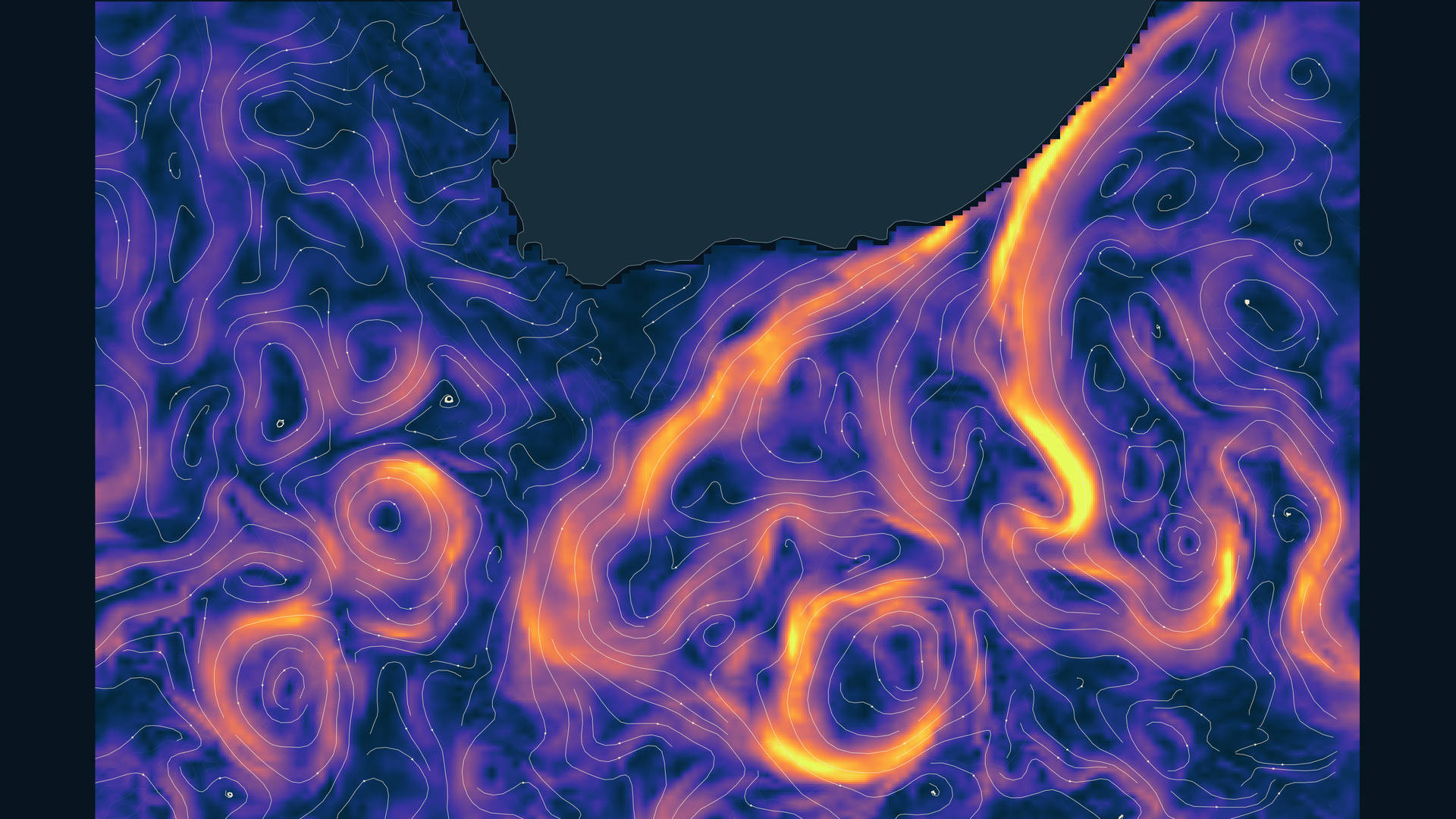
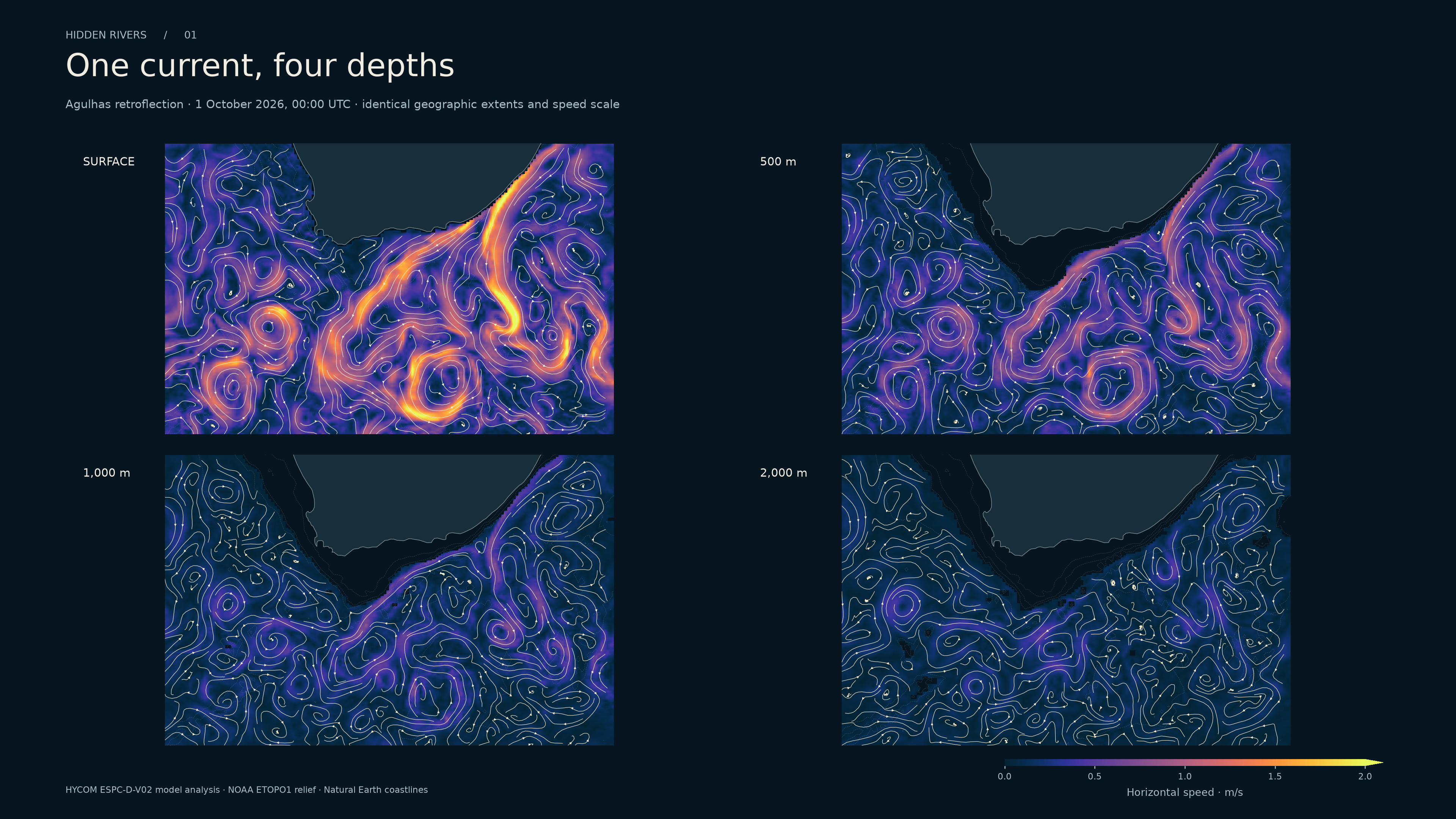
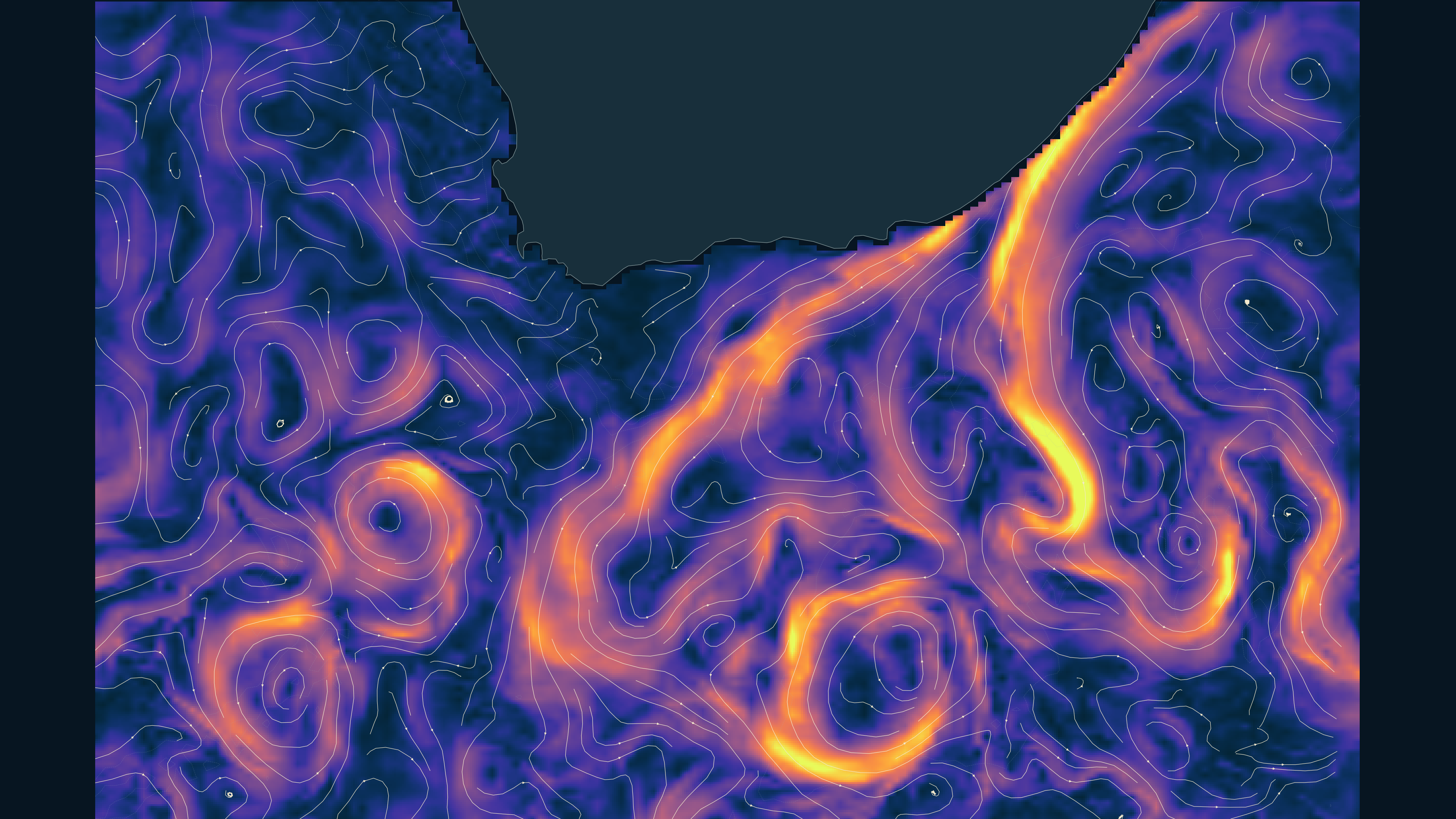
Agulhas retroflection
One current, four depths
The Agulhas turns south of Africa. Hold the geography and the speed scale fixed, then move down through the water column. A strong surface jet need not occupy the same place, or carry the same speed, a kilometre below it.
Horizontal speed · m/s

HYCOM ESPC-D-V02 model analysis · 1 October 2026, 00:00 UTC
Sources and interpretation
These are horizontal, instantaneous model streamlines at fixed depths. They show neither descending water nor measured parcel tracks. NOAA seabed contours provide context. Every depth uses the same 0–2 m/s scale; faster cells use its top color.
Exact grids, checksums and processing ↗Images are exported at 3,840 × 2,160 pixels. Map colors use linear display interpolation within valid source cells; the section retains native cells. The export size does not create finer source detail.
Ocean calculations, films and earlier maps ↗
DENSITY & ROTATION
Dye & vortices
A denser drop sinks and sets the surrounding water turning. Follow the dye, or choose Vorticity to see the rotation in a cross-section.
Dye shows the path of the released water. Switch to Vorticity to see where the flow turns.
Choose an experiment
Set the water and drop
The drop is denser than the water.
Advanced display
Display follows the screen’s refresh rate. Finer uses four times as many cells as the middle setting; a larger salinity difference also takes more computation. Requested pace is reached only when the calculation can keep up.
Drag to turn the tank; scroll or pinch to zoom. Tap to add dye on the release plane. Choose “Pour dye” for continuous drops. Water and resolution changes start a new tank.
Gold marks a saltier or matching addition; coral marks a fresher one.
Dye starts underwater without a push. A density difference drives the water; the dye follows it. In stratified water, a plume can spread sideways near a layer of similar density. Turn the view to see motion through the tank’s full depth.
What the physics includes
Three-dimensional incompressible Boussinesq flow runs entirely in your browser, with velocity in all three directions. Salt and both pigments use conservative cell-face transfers. Half-step transport before and after the velocity update keeps the density response centered in time. TEOS-10 supplies standard-composition seawater density at 10 °C and atmospheric pressure; the controls use Absolute Salinity in g/kg. Glass sides and bottom resist sliding. The flat top is a rigid lid with zero shear.
Resolution controls change the actual calculation: 32³, 64 × 32 × 32 or 64³ cells. The finest grid has 3.75 × 2.81 × 2.81 mm cells. Where WebGPU is available, momentum transport uses single precision on the GPU; density, pressure and conservative salt/dye transfers remain in double precision. Other devices use the double-precision reference calculation. Limited transport reduces smearing; it cannot resolve molecular mixing, turbulent entrainment or a drop striking a free surface. Temperature and viscosity are held fixed. The simulated clock can run more slowly on a finer grid or slower device.
The 3D display traces light through the calculated volume and blends a short queue of computed frames at the screen’s refresh rate. Smooth display motion can continue while the simulated clock runs more slowly. The cross-section samples one physical plane; its slider also places new drops. Cyan and coral show opposite turning directions on that plane, with x right and y down. Drawing resolution adjusts to device performance. WebGL integrates pigment attenuation along the view and light rays to reveal folds and depth. The optical coefficients, colors, lighting and glass are artistic; interpolation adds no physical detail. Salinity uses 0–40 g/kg and flow speed 0–50 mm/s display scales. Vorticity is the curl of the calculated velocity: strength uses 0–8 s⁻¹; signed depth-axis rotation uses −8 to +8 s⁻¹. The signed colors use a square-root stretch to make weaker rotation visible; the endpoints clip. This diagnostic adds no force. Stable-layer, conservation, symmetry, pressure and replay checks accompany grid, timestep and GPU comparisons. Time coupling ↗ · Vorticity method ↗ · Equations ↗ · Reference results ↗ · GPU method ↗ · GPU comparisons ↗
TEOS-10 seawater density ↗ · Bridson's fluid simulation notes ↗
FOR A CONVERSATION
Does the bright surface current stay in the same place at 1,000 m?
Talking points
Compare its position and brightness using the unchanged map and color scale. A depth slice tells us about horizontal motion there; it cannot tell us how water travels between the slices.
Change one water property
Seawater density at the surface, calculated with TEOS-10.
Salt and temperature change together in the real ocean. This controlled calculation holds pressure and the reference location fixed; it does not simulate sinking or mixing.
WHAT THE NEXT MAPS NEED TO SHOW
Following the water to the seabed
Denmark Strait: a descending plume
A map alone hides the important geometry. Pair the roughly 650 m sill and seabed with ship sections of temperature, salinity, density and velocity at the sill. A separate downstream layer would show descent and mixing, distinguishing its observations from model output. The existing 1,000 m map cannot reconstruct that descent.
Sill observations: Lin et al. (2020) ↗Downstream observations and model: Käse et al. (2003) ↗
Research direction. Public mooring records are available; a downloadable set of the complete gridded ship sections has not yet been verified.
Ross Sea: the surface signature of deep water
Dense shelf water leaves through seabed troughs. A 2025 study used ocean models to test a sea-surface-height proxy, then compared satellite variability with hydrographic evidence. A useful image would put the deep plume, the surface signal and the sampling gaps beside one another.
Altimetry study: Auger et al. (2025) ↗Research direction. Figure data are openly archived; reconstructing the observation-based proxy requires the along-track altimetry and the published filtering and coverage criteria.
Congo Canyon: sediment makes a gravity current
Suspended sediment can make water dense enough to travel down a submarine canyon. Moorings and cable-break times documented a January 2020 current that travelled more than 1,100 km and accelerated along its route. A reconstruction could map those measured arrival times against the canyon.
Measured canyon flows: Talling et al. (2022) ↗Research direction. Sensor coverage, interval-averaged front speeds and multibeam coverage must remain visible in a reconstruction.
Denmark Strait carries a bottom-following overflow, and the Gulf Stream also has a major wind-driven component. Satellites measure surface signals; they do not photograph deep currents. Popular descriptions of underwater waterfalls and conveyor belts simplify these different processes. Introductory overview ↗ · WHOI's explanation ↗