IAN HELFRICH / OCEANOGRAPHIC SYSTEMS
Hidden Rivers
The ocean’s submerged currents.
HYCOM · NOAA · Tessera · Cesium
The map roomLoading ocean fields
Horizontal flow in the ocean interior
01 / LAGRANGIAN TRANSPORT
Follow a parcel through a changing current.
Each filament is a numerical trajectory through the model’s evolving horizontal velocity field. Its history is measured in ocean hours, independent of the display’s frame rate. Scrubbing time follows the same seeded particles.
Particles stay on a selected depth surface. These paths do not include vertical motion, turbulent diffusion, waves, or windage.
VELOCITY / SELECTED LOCATION
Choose a location in the ocean.
| Depth | Speed | East | North | Toward |
|---|---|---|---|---|
| Click the field above or enter coordinates. | ||||
Directions point toward motion, clockwise from true north. Missing values remain missing. Depth colors identify the plotted series; they do not encode speed.
SATELLITE SCENES / OCEAN COLOR / COASTLINES
The ocean,
in its own colors.
Satellite views set beside measured ocean fields. Each image keeps its date, spatial scale, source, and limits in view.
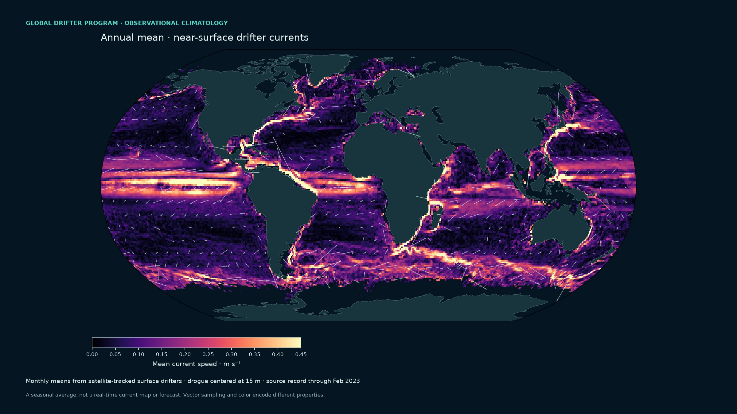
The currents that wrap the world
A global seasonal view derived from observed drifting-buoy velocities, with the drogue centered at 15 m. This is a climatology through February 2023, not a real-time map. Animated particles trace the mean fields for illustration; they are not measured drifter tracks.
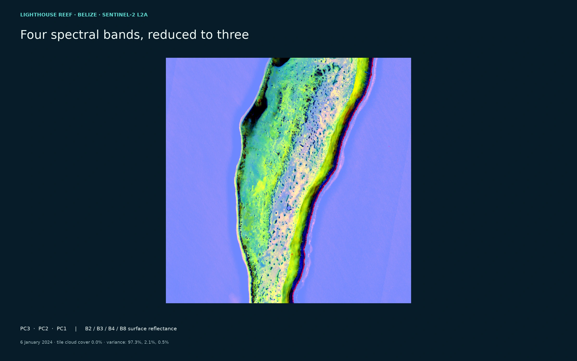
Light through four bands
True PCA of cloud-screened Sentinel-2 surface reflectance: blue, green, red, and near-infrared. PC3 / PC2 / PC1 are shown as RGB; stretch is percentile-based. This is spectral structure, not a coral-health classification.
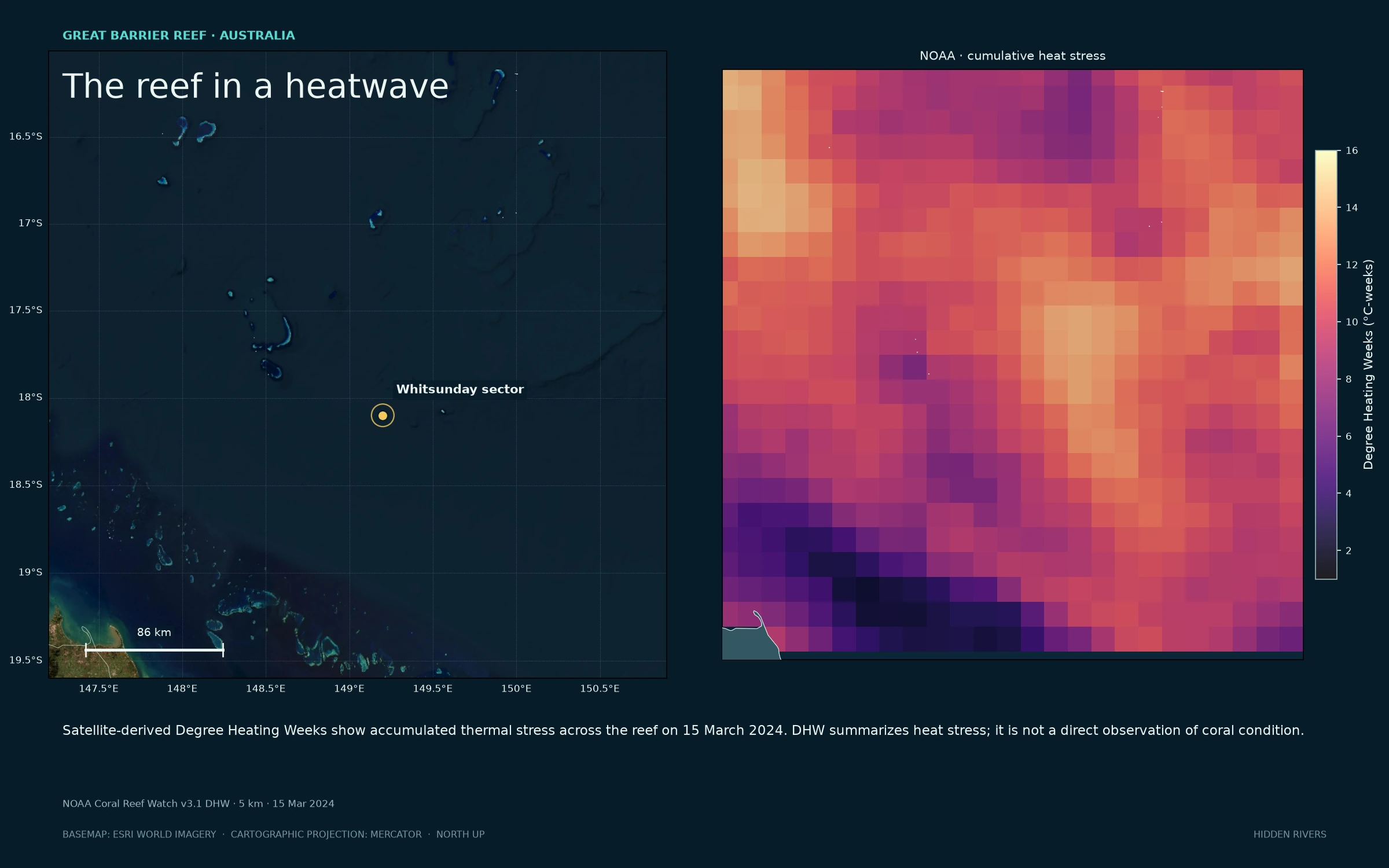
Heat held in the reef
Great Barrier Reef, with NOAA’s satellite-derived cumulative heat stress beside the natural-color scene. The colors describe thermal exposure, not observed coral condition.
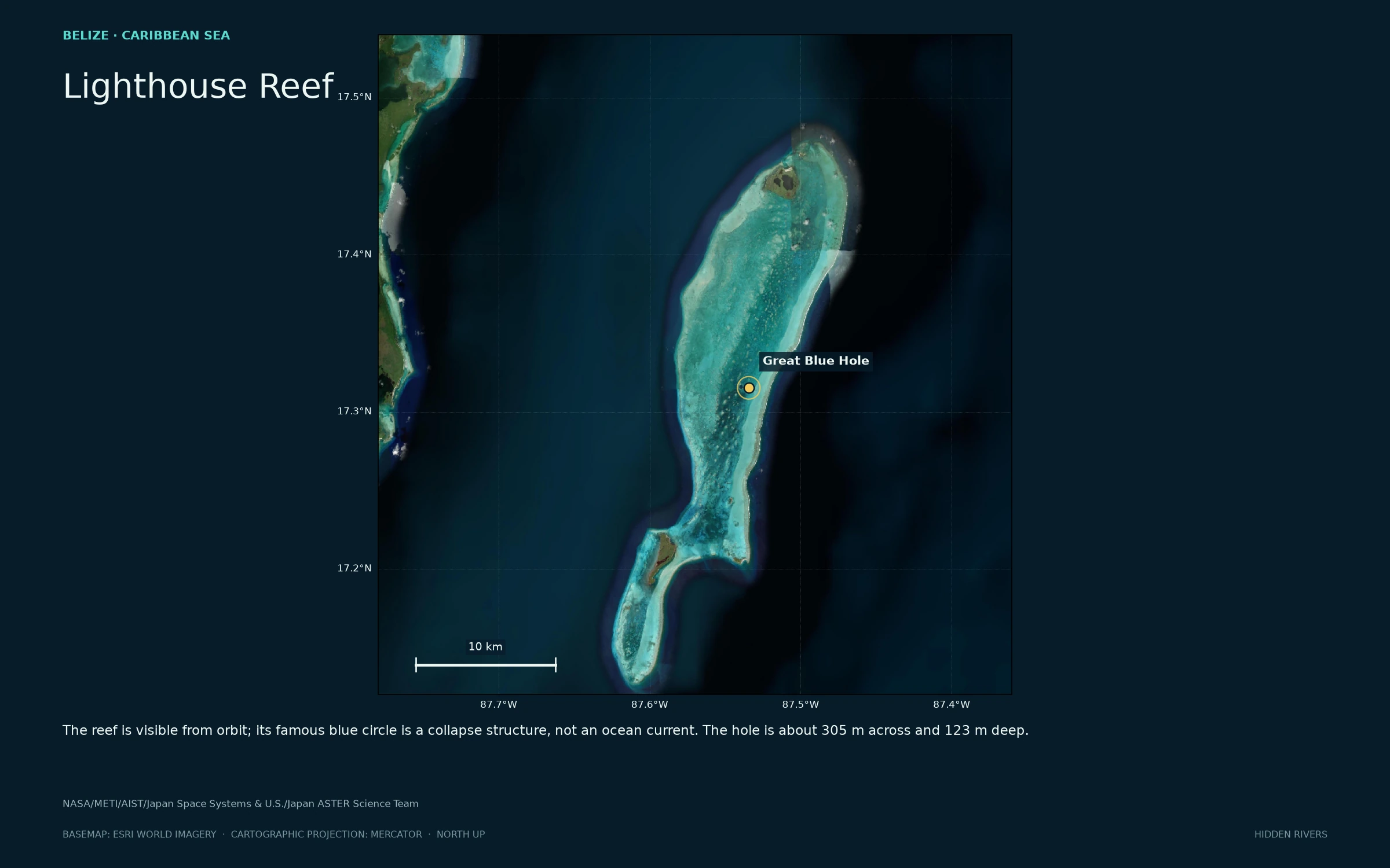
The Blue Hole, held in the reef
Aerial context for the circular collapse feature and its surrounding atoll.
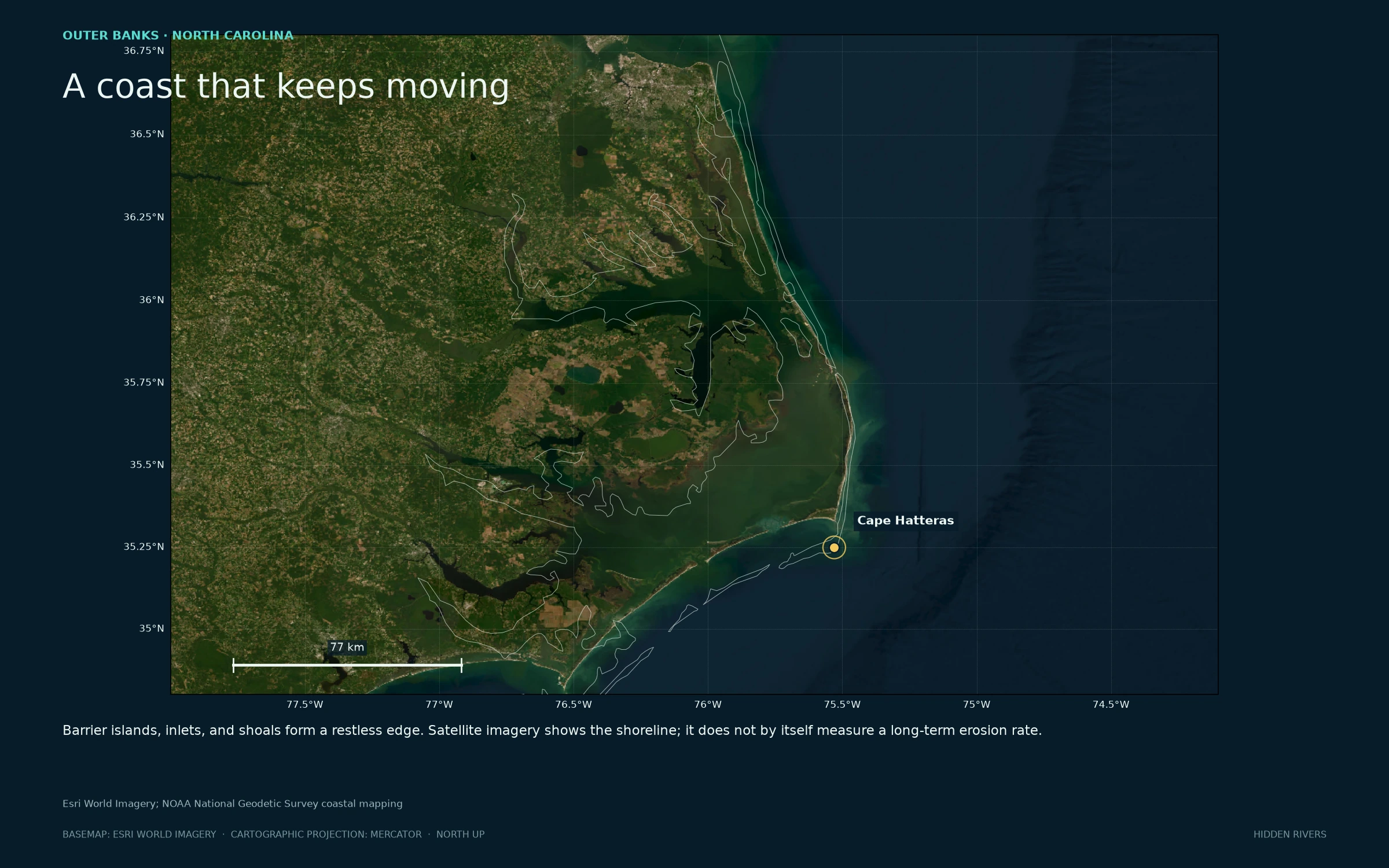
Outer Banks, shifting edge
Barrier islands, inlets, and shoals. This scene is geographic context, not an erosion-rate estimate.
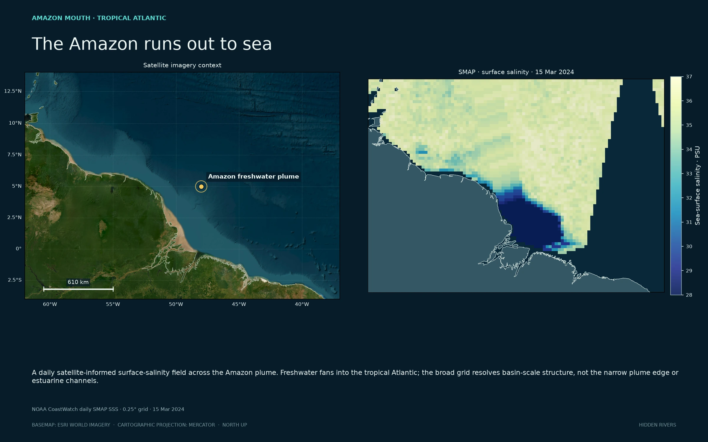
Fresh water meeting salt
Amazon plume imagery alongside one NOAA SMAP daily surface-salinity field at its native 0.25° grid. Near-land retrievals are less reliable; this broad view does not resolve estuaries.
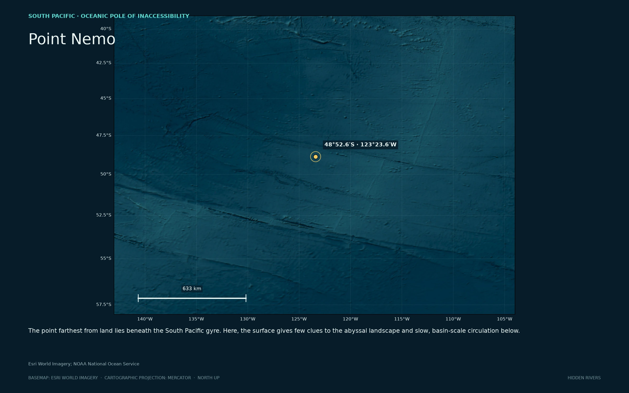
Water in every direction
Point Nemo sits far from land beneath the South Pacific gyre.
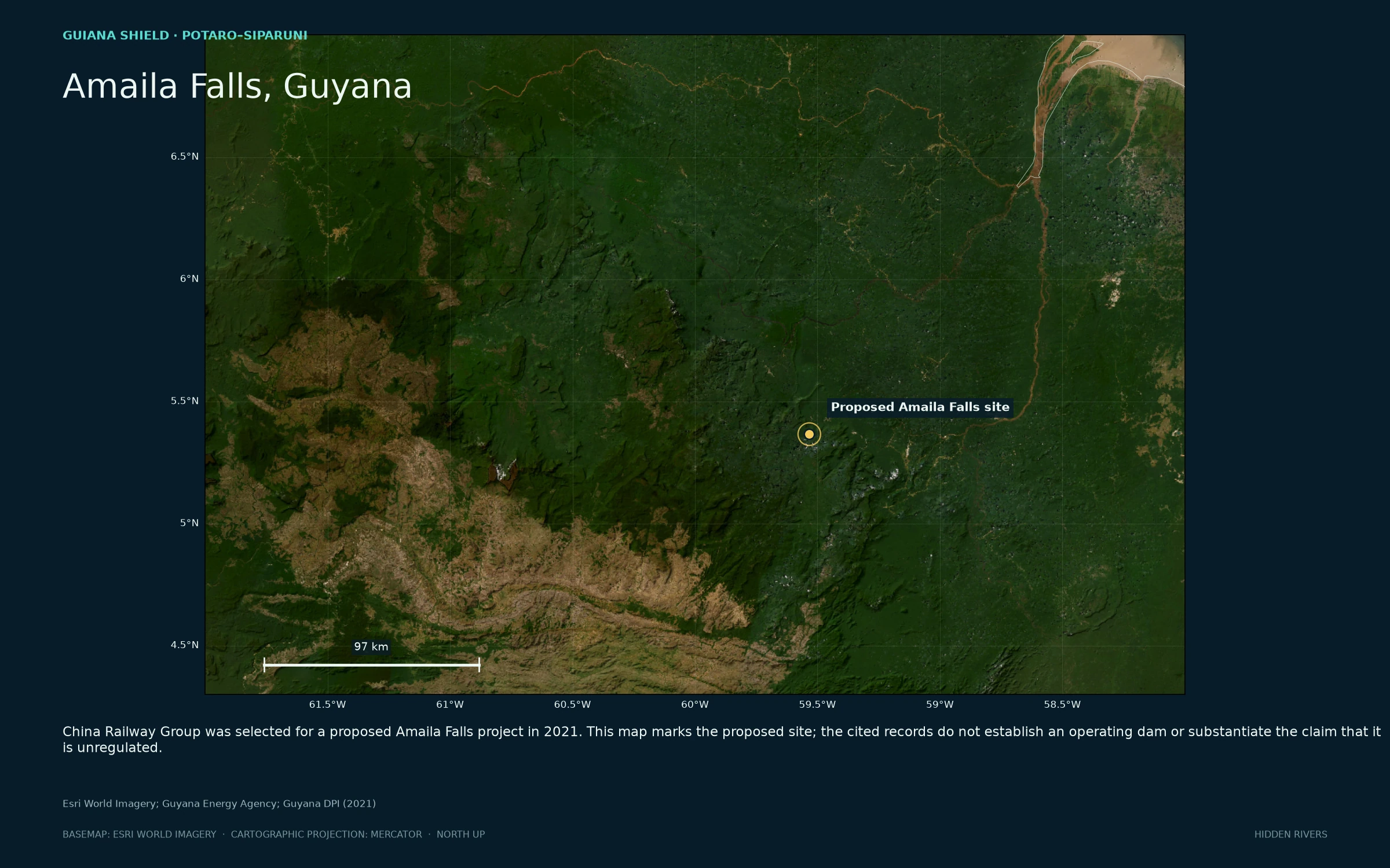
Amaila Falls, Guyana
Forest and river country around the proposed site. The cited government records do not establish an operating dam or that it is unregulated.
Satellite basemap: Esri World Imagery (imagery dates vary). PCA input: Copernicus Sentinel-2 Level-2A, 10 m bands; colors are principal components, not natural color. NOAA SMAP salinity is a daily satellite-informed Level-3 field on a 0.25° grid. NOAA Coral Reef Watch DHW is a 5 km satellite-derived thermal-stress product.
SIX MAPS / DOWNLOADABLE AT 2,800 × 2,000
Model fields
in stills.
Current direction, speed, rotation, and stretching come from the released HYCOM fields. Every plate includes its own scale, date, depth, and projection.
Presentation mode: ← → to change visuals · Space to pause · Esc to return. Move the pointer or tap for controls.
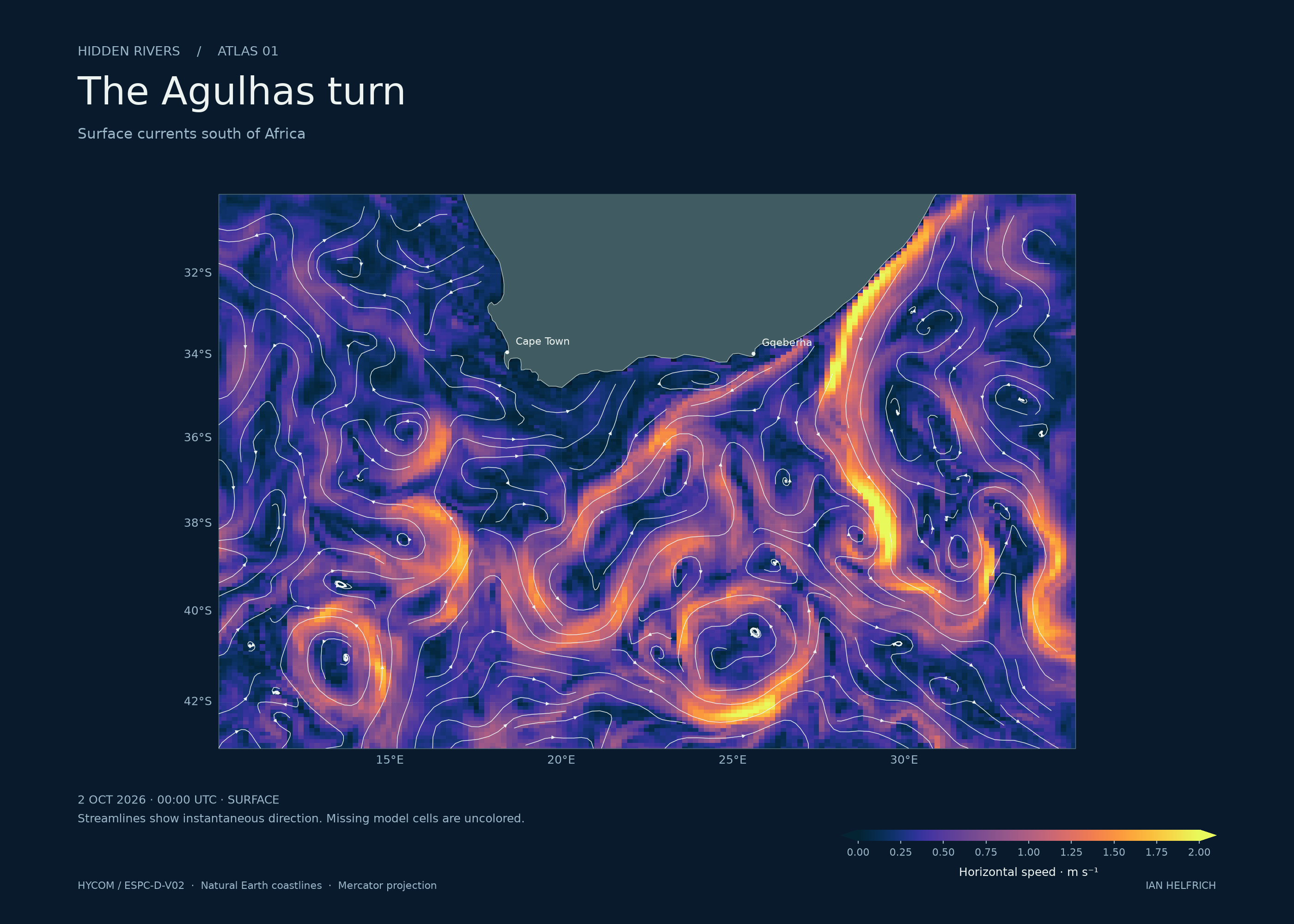
The Agulhas turn
Surface currents south of Africa
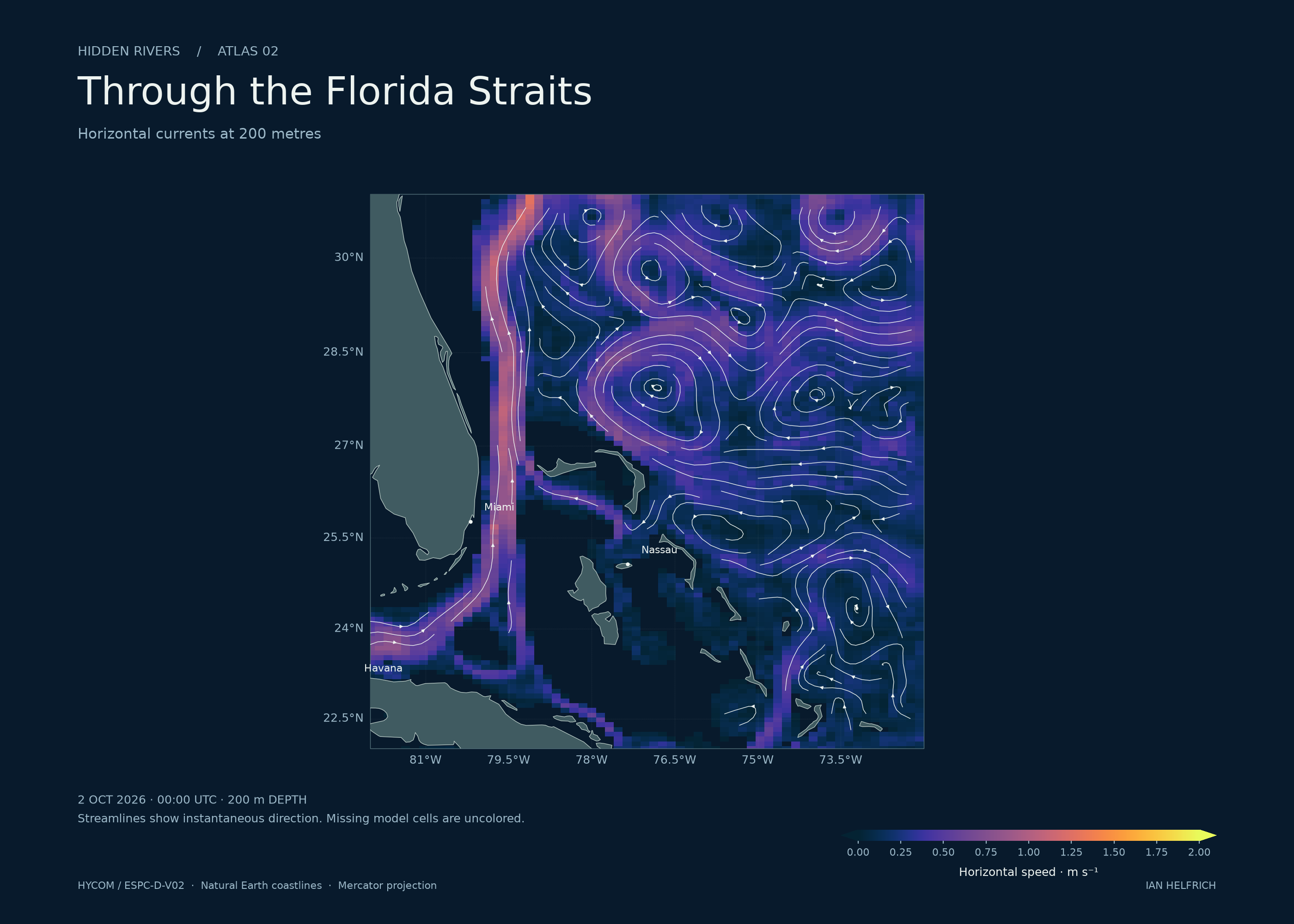
Through the Florida Straits
Horizontal currents at 200 metres
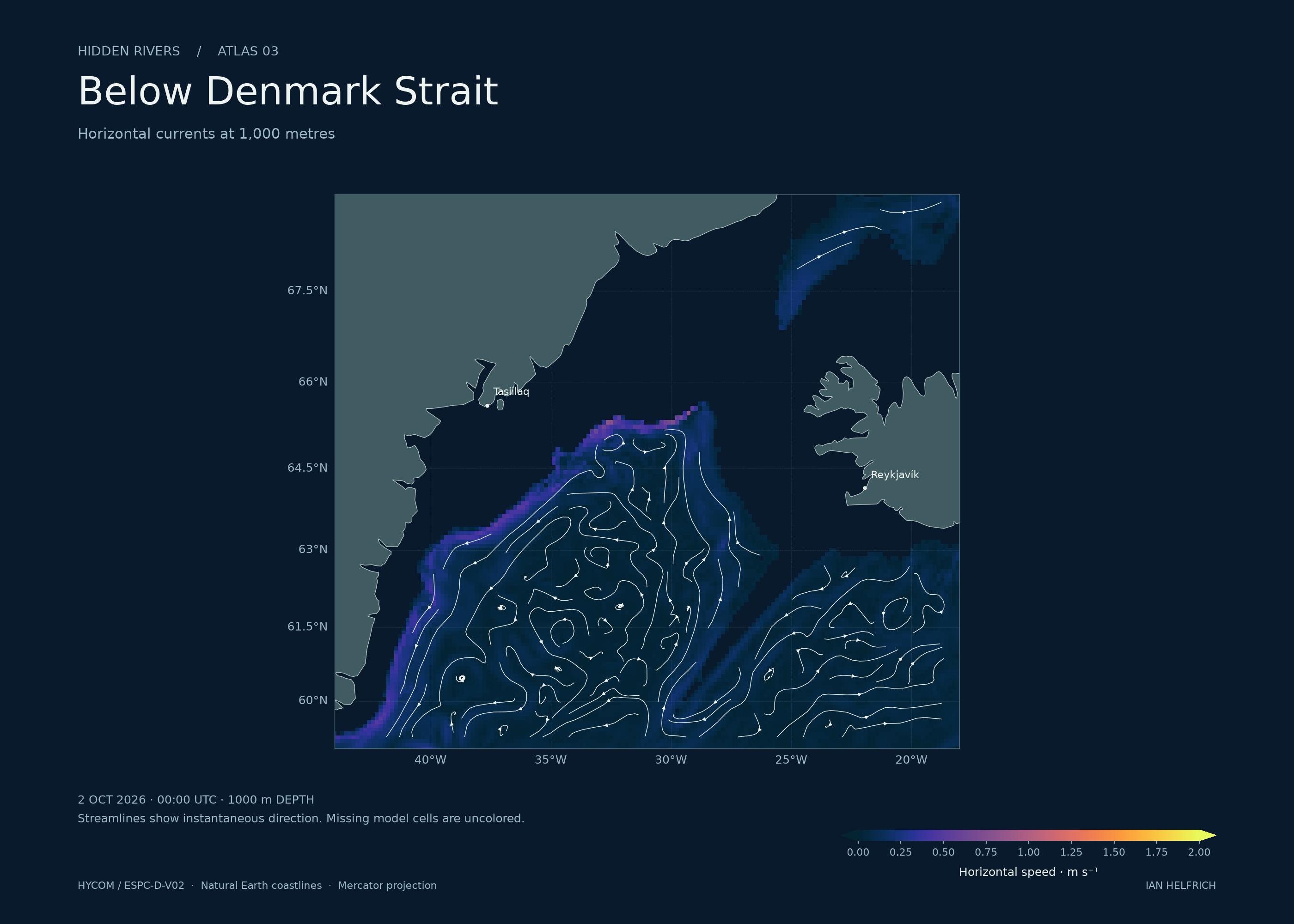
Below Denmark Strait
Horizontal currents at 1,000 metres
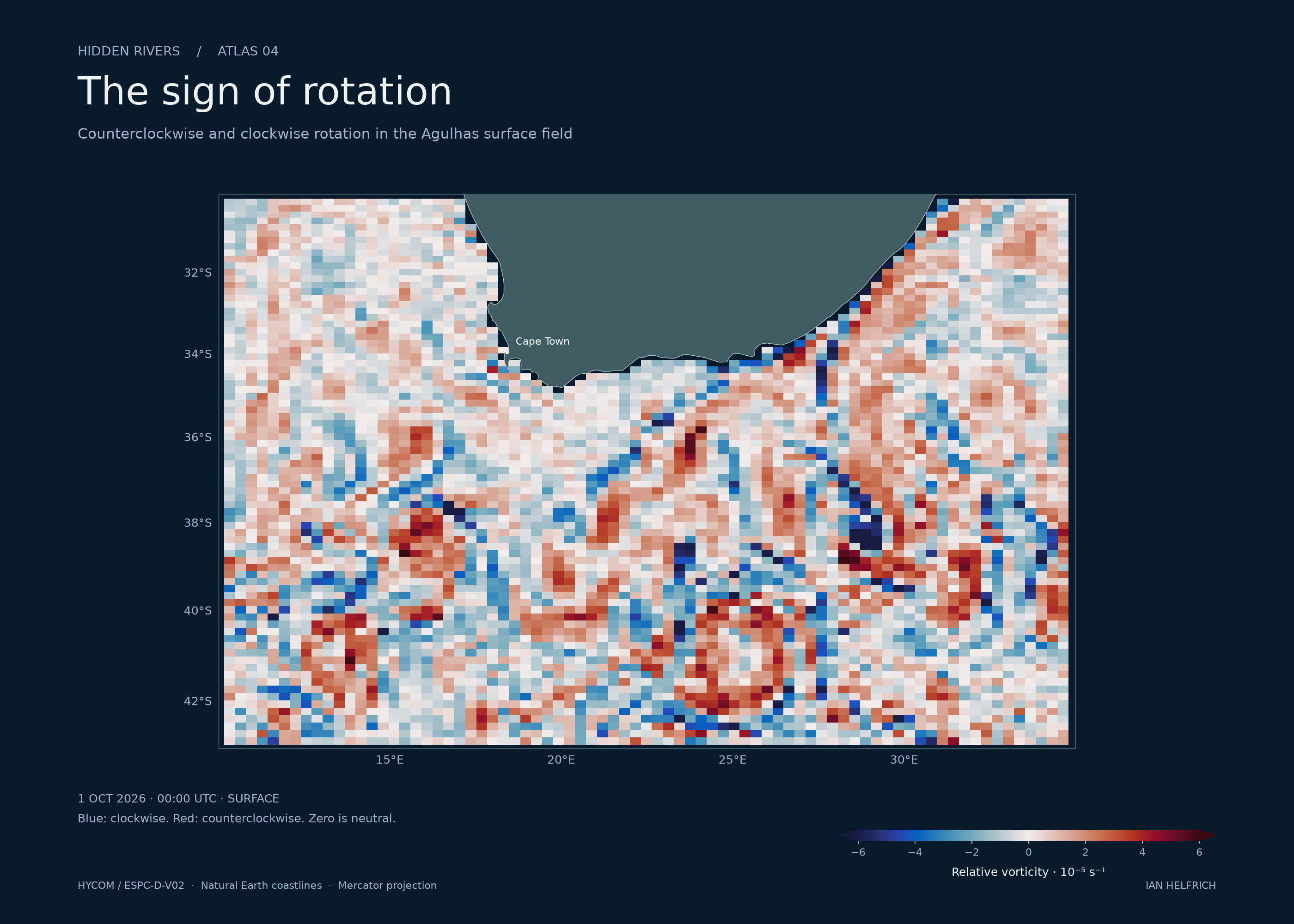
The sign of rotation
Clockwise and counterclockwise surface rotation
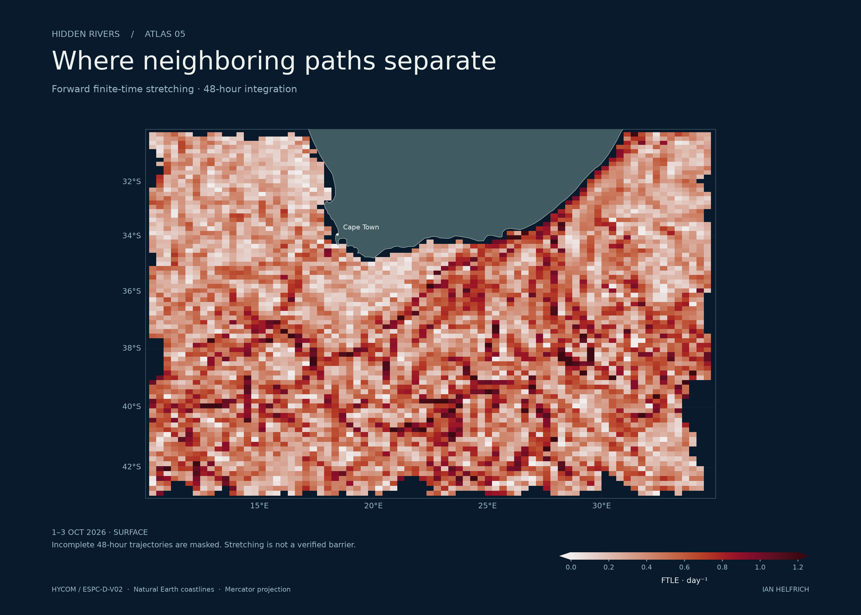
Where neighboring paths separate
48-hour forward stretching, 1–3 October 2026
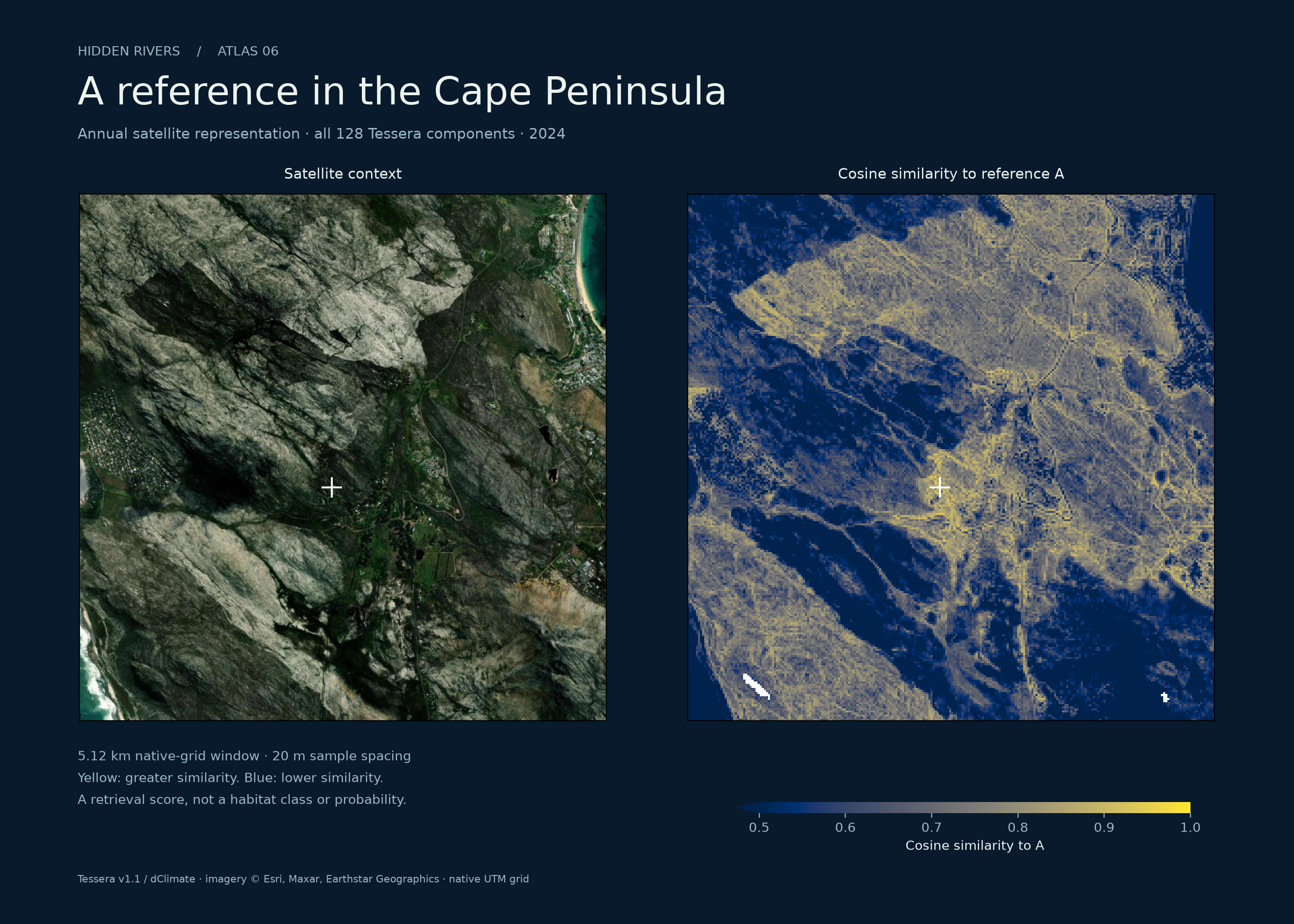
A reference in the Cape Peninsula
2024 Tessera similarity beside satellite context
24 PLACES / CESIUM WORLD TERRAIN & OSM BUILDINGS
Rivers meet
the built world.
From Fayetteville on the Cape Fear to the mountains above Cape Town. Terrain and available building geometry give the landscape its shape; aerial imagery supplies surface detail.
Cape Fear River and downtown Fayetteville. This inland river city is upstream of Wilmington.
78.88° WFAYETTEVILLE / CAPE FEAR RIVER
Building coverage and height detail vary by location. These 24 camera destinations provide geographic context. The ocean model covers three regions; the Tessera sample below covers the Cape Peninsula.
02 / TESSERA REPRESENTATIONS · CAPE PENINSULA · 2024
The Cape Peninsula
in 128 dimensions.
Select a reference on the coast. Tessera’s full feature vector becomes a spatial query: which other locations resemble it in the satellite representation?
Use a second reference to inspect the difference. The colors show similarity or preference between references, with an explicit numerical scale.
The coastal representation loads when this section enters view.
03 / CURRENTS IN MOTION
A year of ocean flow.
A text-free seasonal loop through NOAA’s monthly mean currents from satellite-tracked drifters. The drogue sat at 15 m. The colors show annual-mean speed; particles follow a visual integration through the climatology, not individual observed drifters. This is a long-run seasonal pattern, not today’s ocean.
THE AGULHAS · HYCOM · 0 M
One day along the current off southern Africa.
A regional model view with the ocean surface kept level. Trails show horizontal motion only; particle count is not transport volume.
Download Agulhas film ↗04 / METHODS & EVIDENCE
Data and
calculations.
The ocean model supplies eastward and northward velocity at geographic coordinates and depth. The atlas turns those fields into three distinct calculations. A path describes where a tracer travels; vorticity describes local rotation; finite-time stretching describes separation of nearby trajectories over a stated interval.
None is a direct observation of every parcel. The model grid, input cadence, missing values, and integration window constrain the result. Smaller integration steps improve the numerical calculation, not the resolving power of the source data.
01 Geographic particle trajectories +
Longitude λ and latitude φ are in radians; u and v are in metres per second. The renderer uses deterministic releases and a fixed physical sampling interval for trajectory history. The same model time therefore produces the same path geometry across devices. Masked cells and exits terminate trajectories.
Depth remains fixed at the selected model level. The oblique view uses the same horizontal and vertical scale, so deep layers sit close together. A 20 m rendering offset keeps paths legible against the surface. Particle number, glow, and line density aid visibility and do not represent transported volume or probability. NOAA relief and the model’s wet mask are independently gridded and can differ near slopes.
02 Rotation on a sphere +
Relative vorticity has units of inverse seconds. Positive values describe counterclockwise local rotation; negative values describe clockwise rotation. A diverging palette places zero at its center. This diagnostic is a finite difference of the model field; it does not by itself identify a persistent eddy.
03 Finite-time stretching +
The flow map Φ moves nearby initial locations through 48 hours of velocity data. Its spatial derivative measures how those locations separate. The largest stretching direction gives the forward finite-time Lyapunov exponent, reported per day. Trajectories without a valid full integration window are masked.
High stretching can arise from shear as well as features associated with coherent transport. A bright ridge is not proof of a transport barrier. The published diagnostics include numerical sensitivity checks; they do not quantify all ocean-model uncertainty.
04 Similarity across all Tessera dimensions +
Each vector contains 128 learned features. The microscope compares these vectors by cosine similarity. Positive contrast means the location resembles reference A more than B in this representation. It does not certify habitat type, ecological health, water depth, or current velocity.
The annual coastal representation and ocean analysis have different dates and purposes. Their link is geographic. No predictive or causal relationship between embeddings and currents is claimed.
A MEASURED LIMIT / AGULHAS SURFACE
The sampling interval changes the answer.
For the same 48-hour calculation, switching from three-hour inputs to daily samples changes the stretching field much more than halving the integration step. Small numerical error does not establish physical accuracy.
Absolute FTLE differences are in day⁻¹. Each comparison uses seed/window pairs valid in both runs across four release dates. These are sensitivity checks, not observational error estimates.
| Changed setting | Median | 95th percentile | Pairs |
|---|---|---|---|
| Inputs: 3 hours → 24 hours | 0.113692 | 0.427221 | 1,231 |
| RK4 step: 900 s → 450 s | 0.00000462 | 0.00005767 | 1,238 |
| Perturbation: ¼ → ⅛ cell | 0.008695 | 0.056488 | 1,238 |
The Depth view uses daily inputs for all five Agulhas layers. Surface-only transport and diagnostics retain the three-hour series. The six other velocity layers have daily inputs.
Inputs
HYCOM / ESPC-D-V02 ↗NOAA Global Drifter Program climatology ↗NOAA ETOPO1 relief ↗Tessera / GeoTessera ↗Cesium ion terrain & buildings ↗Inspect the release
Velocity metadata ↗Diagnostic metadata ↗Daily source requests ↗Three-hour source requests ↗500 m & 2,000 m source requests ↗Tessera provenance & validation ↗Analysis, tests & rendering code ↗Interpretation
FTLE uncertainty: Matuszak et al. ↗WHOI: circulation and eddies ↗Research visualization. Physical validation against colocated observations remains outside this release.