16 Workbook · Hypothesis testing in practice
- Setting up null and alternative hypotheses for a real question
- Choosing the right test (one-sample, two-sample, paired, proportion, chi-squared)
- Computing test statistics and reading p-values honestly
- Distinguishing statistical from practical significance
- Reasoning about Type I and Type II error rates and power
Hypothesis testing is a procedure for asking “could this result have happened by chance?” The procedure has five parts that recur in every test:
- State the null hypothesis H_0 and the alternative H_1.
- Pick a test statistic and a significance level \alpha (conventionally 0.05).
- Compute the test statistic from the data.
- Compute the p-value: the probability, under H_0, of seeing a test statistic at least as extreme as the one you computed.
- Reject H_0 if p < \alpha, otherwise fail to reject.
The eight problems below walk through different testing scenarios, each with the full five-part structure. Solutions show working, not just answers. The skill is recognizing which test fits which question and reading the result honestly, including its limitations.
16.1 Problem 1: One-sample t-test
A manufacturer claims its production process produces parts with mean weight 100 grams. You sample 25 parts at random. Their mean weight is 102.3 g with sample standard deviation 4.5 g. At \alpha = 0.05, is the manufacturer’s claim consistent with your data?
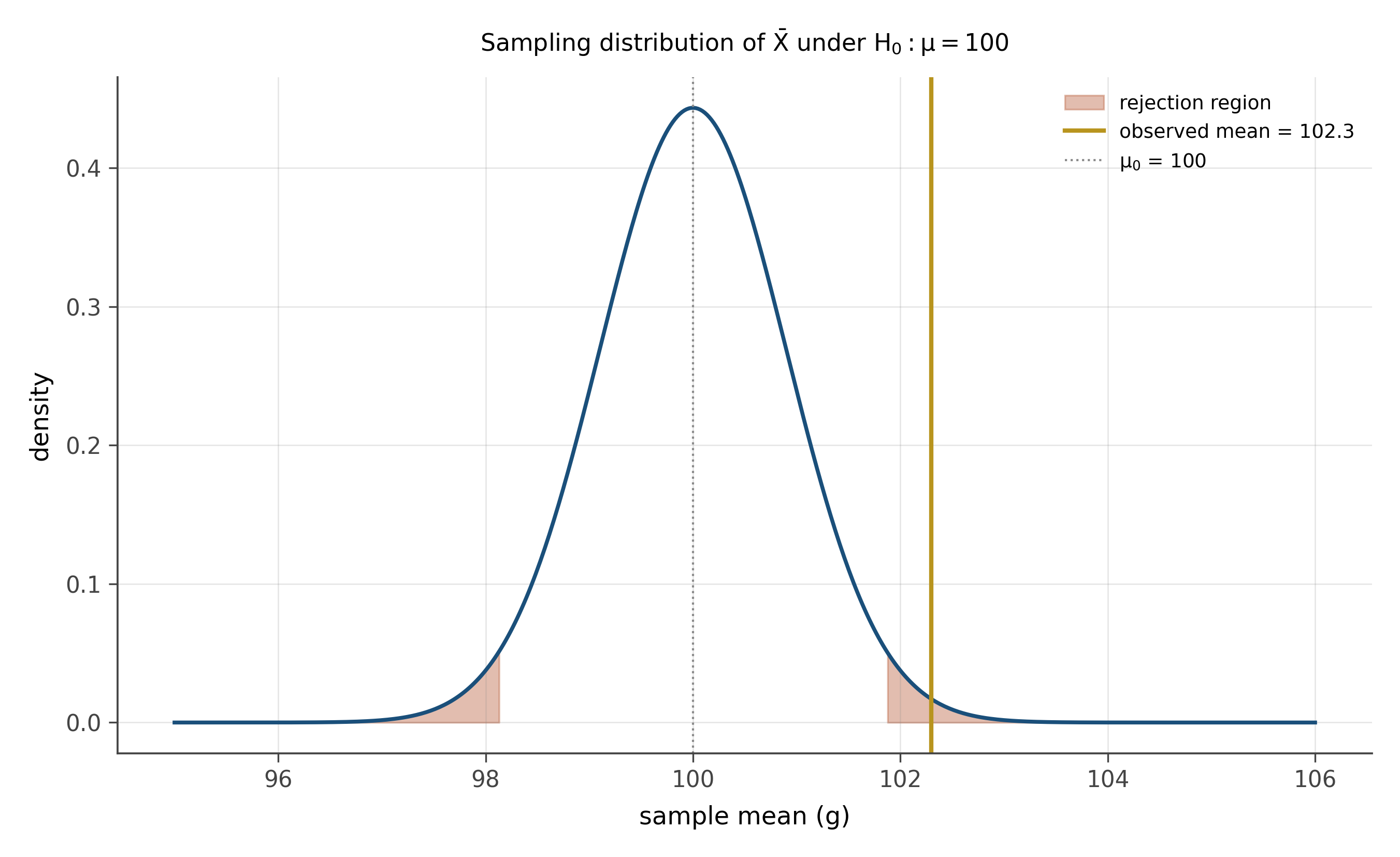
Setup. H_0: \mu = 100. H_1: \mu \neq 100 (two-sided, since we have no prior reason to expect the true mean to be larger or smaller). \alpha = 0.05.
Test statistic. A one-sample t-statistic: t = \frac{\bar{x} - \mu_0}{s / \sqrt{n}} = \frac{102.3 - 100}{4.5 / \sqrt{25}} = \frac{2.3}{0.9} \approx 2.56.
Reference distribution. Under H_0, t follows a Student’s t distribution with n - 1 = 24 degrees of freedom.
P-value. Two-sided. The critical t-values at \alpha = 0.05 with 24 df are \pm 2.064. Our observed t = 2.56 is more extreme than 2.064. The two-sided p-value is approximately 0.017 (which you can check with pt(-2.56, 24)*2 in R or 2*(1 - stats.t.cdf(2.56, 24)) in scipy).
Decision. Reject H_0. The data are inconsistent with the manufacturer’s claim of mean weight 100 g, at the 5% level.
A note on practical significance. Statistical significance does not equal practical significance. The estimated effect size is \bar{x} - \mu_0 = 2.3 grams, or 2.3% of the claimed mean. Whether that is practically meaningful depends on the application. For pharmaceutical doses, 2.3% might matter. For shipping packages, it might not. Always report both the effect size and its uncertainty, not just the p-value.
16.2 Problem 2: Two-sample t-test
A new drug is supposed to reduce systolic blood pressure. You randomize 80 hypertensive patients to drug or placebo (40 each). After 12 weeks, the drug group has mean SBP 138 mmHg with s = 12. The placebo group has mean SBP 145 with s = 14. Is the drug effective?
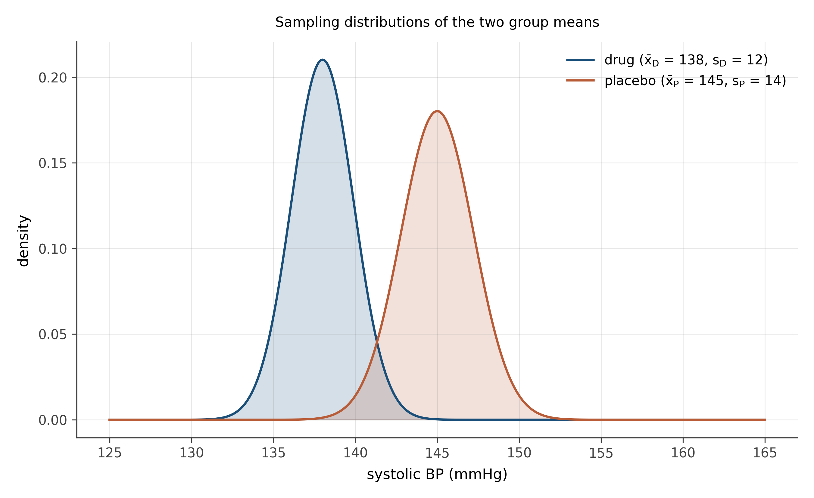
Setup. Let \mu_D = mean SBP under drug, \mu_P = mean SBP under placebo. H_0: \mu_D = \mu_P. H_1: \mu_D < \mu_P (one-sided, because the only clinically meaningful direction is “drug lowers BP”). \alpha = 0.05.
Test statistic. Two-sample t assuming unequal variances (Welch’s t-test, the safe default): t = \frac{\bar{x}_D - \bar{x}_P}{\sqrt{s_D^2 / n_D + s_P^2 / n_P}} = \frac{138 - 145}{\sqrt{144/40 + 196/40}} = \frac{-7}{\sqrt{8.5}} \approx -2.40.
Reference distribution. Welch’s t, with degrees of freedom approximated by the Welch-Satterthwaite formula. With n_D = n_P = 40 and similar variances, df \approx 76.
P-value. One-sided. Pr(t \leq -2.40 \mid H_0) \approx 0.009.
Decision. Reject H_0. The data support the conclusion that the drug reduces SBP, at the 5% level.
Effect size. \bar{x}_D - \bar{x}_P = -7 mmHg. Cohen’s d \approx -7 / \sqrt{(s_D^2 + s_P^2)/2} \approx -0.54, a moderate effect by conventional standards. Clinically, a 7 mmHg reduction in SBP is meaningful and would lower cardiovascular risk in a treated population.
Always report both. The 95% confidence interval for the difference is approximately -7 \pm 1.99 \cdot \sqrt{8.5} \approx (-12.8, -1.2) mmHg. Stating this interval is more informative than just the p-value: it tells the reader the plausible range of the true effect, not just that it is distinguishable from zero.
16.3 Problem 3: Paired difference
You measure the cholesterol level of 30 patients before and after 8 weeks of a dietary intervention. The mean within-subject change is -8 mg/dL with standard deviation of changes 14 mg/dL. Did the diet work?
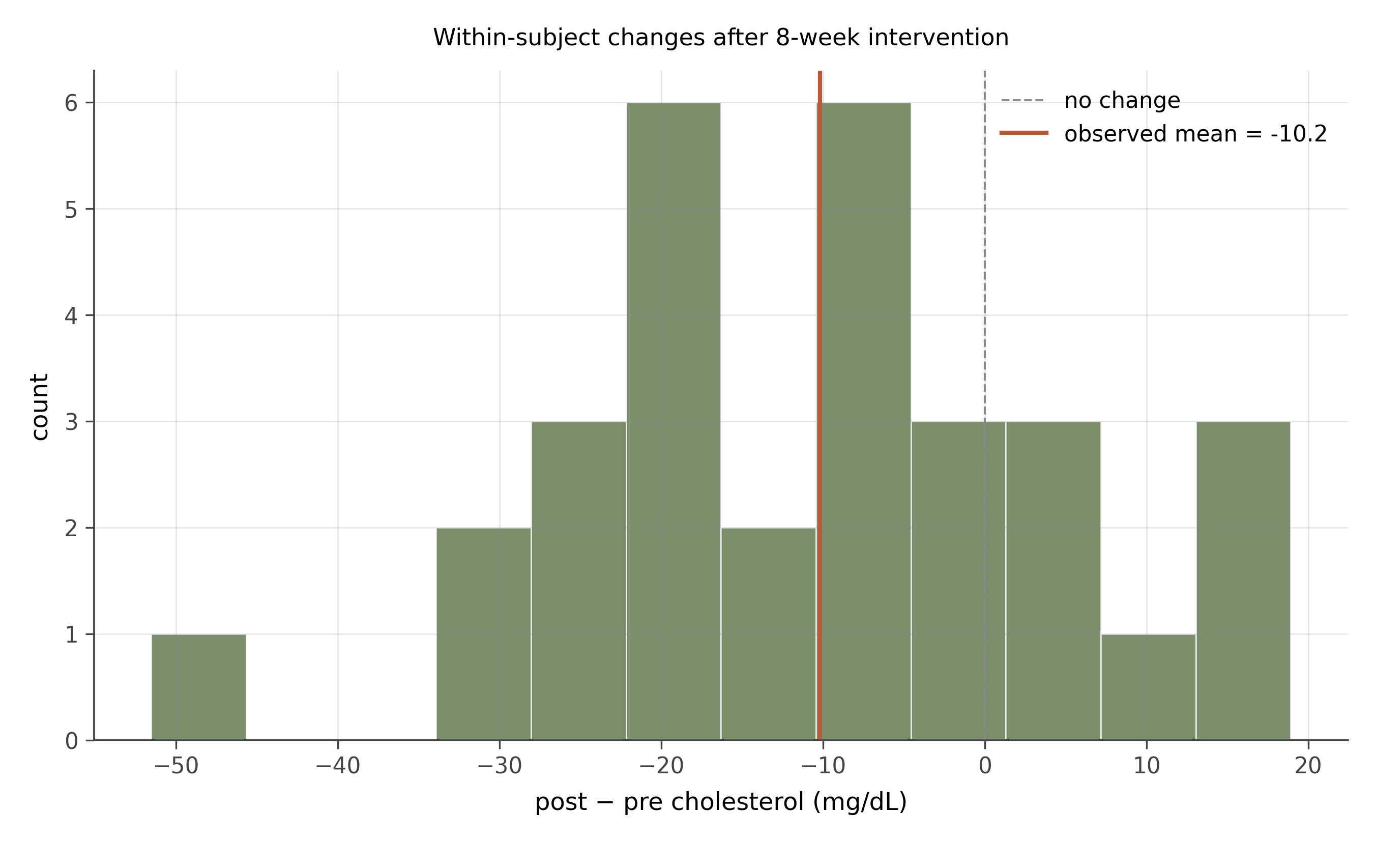
Setup. Let \Delta_i = \text{post}_i - \text{pre}_i for subject i. H_0: E[\Delta] = 0. H_1: E[\Delta] < 0 (one-sided: the diet should lower cholesterol). \alpha = 0.05.
Why paired. Each subject’s pre-measurement is correlated with their own post-measurement. Treating these as independent two-sample data would inflate variance and reduce power. The paired test analyzes the within-subject difference, which removes between-subject variability.
Test statistic. t = \frac{\bar{\Delta} - 0}{s_\Delta / \sqrt{n}} = \frac{-8}{14 / \sqrt{30}} = \frac{-8}{2.56} \approx -3.13.
Reference distribution. Student’s t with n - 1 = 29 df.
P-value. Pr(t \leq -3.13 \mid H_0) \approx 0.002.
Decision. Reject H_0. The intervention significantly reduced cholesterol at the 5% level.
Caveat: causation. The test establishes that mean cholesterol fell among the participants. It does not establish that the diet caused the drop, because there is no control group. Cholesterol could have fallen due to seasonal variation, regression to the mean, the placebo effect, or anything else that would have happened over 8 weeks regardless of the diet. To make a causal claim, you need a randomized comparison group. This is the central distinction Part III will spend chapters on.
16.4 Problem 4: Proportion test
A factory line is supposed to produce no more than 2% defective parts. You inspect 500 parts and find 14 defects. Is the defect rate above the acceptable threshold?
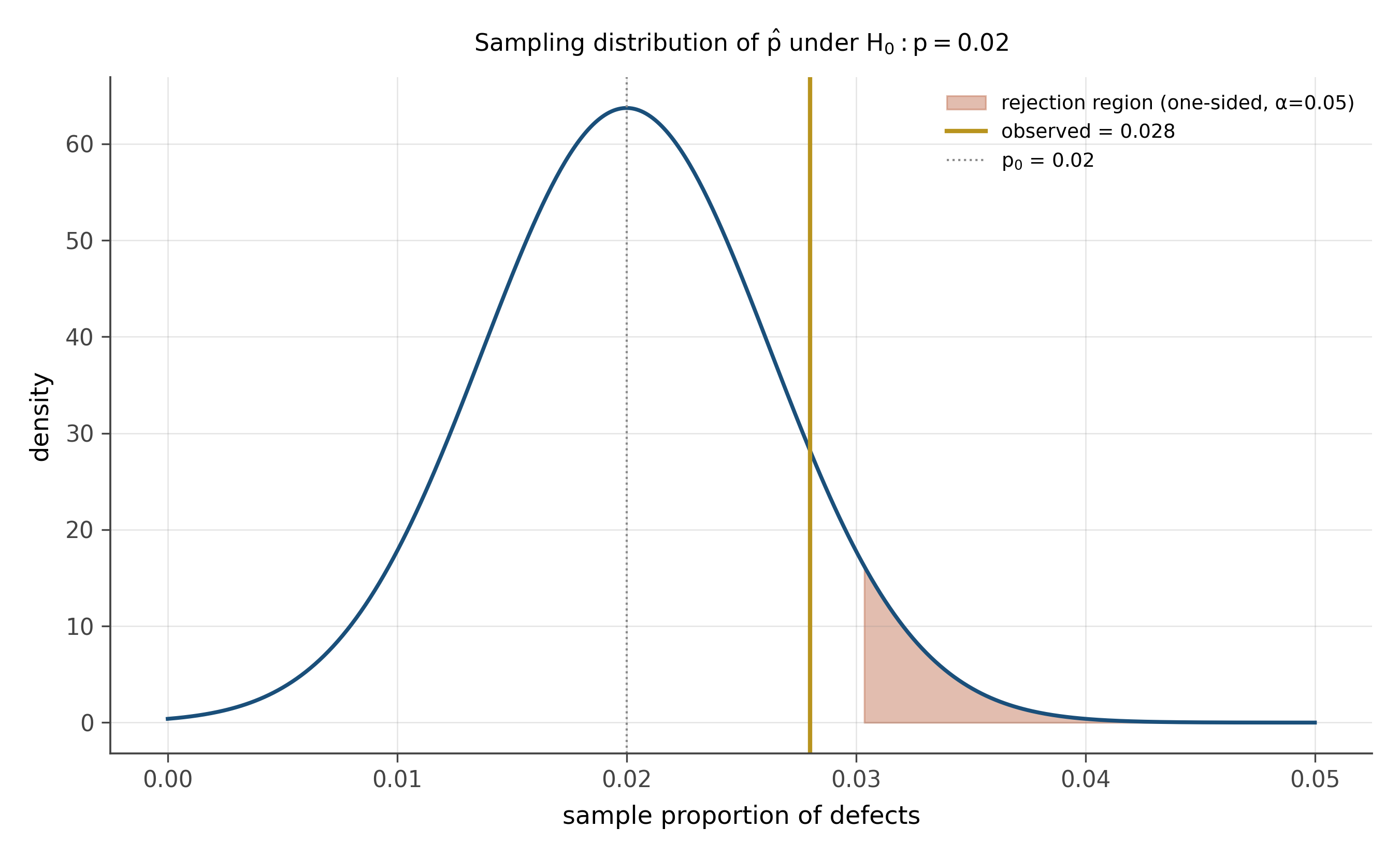
Setup. H_0: p = 0.02. H_1: p > 0.02 (one-sided: we only care if it is too high). \alpha = 0.05.
Sample proportion. \hat{p} = 14/500 = 0.028.
Test statistic. Approximately normal under H_0 when np_0 and n(1-p_0) are both at least 10: z = \frac{\hat{p} - p_0}{\sqrt{p_0(1 - p_0) / n}} = \frac{0.028 - 0.02}{\sqrt{0.02 \cdot 0.98 / 500}} = \frac{0.008}{0.00626} \approx 1.28.
P-value. One-sided. Pr(Z \geq 1.28) \approx 0.10.
Decision. Fail to reject H_0. The data are consistent with a 2% defect rate at the 5% level.
Interpretation. “Fail to reject” is not the same as “accept.” We have not shown that p \leq 0.02. We have shown that the sample of 500 is not large enough to distinguish 2.8% from 2% with confidence. The 95% one-sided upper bound for p is roughly \hat{p} + 1.645 \cdot \text{SE}(\hat{p}) \approx 0.038, so the true defect rate could be as high as 3.8% and still consistent with this sample.
Power. If we genuinely cared about detecting a 2.8% defect rate, this sample size is underpowered. Larger n would shrink the SE and give the test more chance to detect a real elevation. We compute the required n in problem 6.
16.5 Problem 5: Chi-squared independence
A survey of 800 voters asks two questions: party affiliation (Democrat / Republican / Independent) and primary news source (TV / web / print). Are these two variables independent?
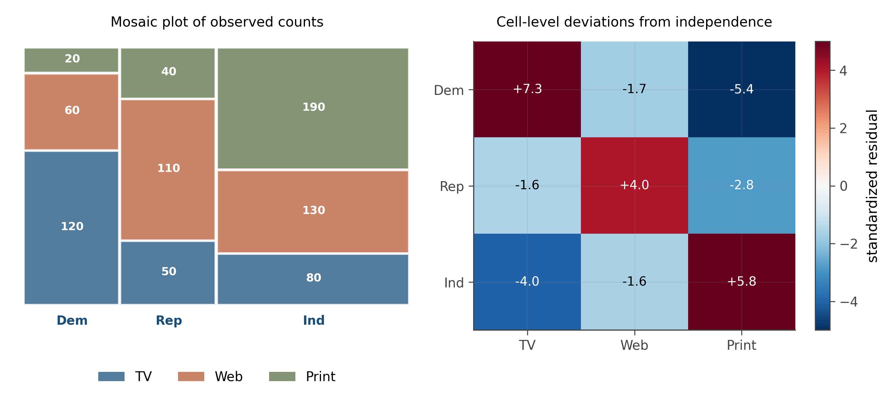
Setup. H_0: party and news source are statistically independent. H_1: they are not. \alpha = 0.05.
Test statistic. Chi-squared: \chi^2 = \sum_{i,j} \frac{(O_{ij} - E_{ij})^2}{E_{ij}}, where O_{ij} is the observed count in cell (i, j) and E_{ij} is the expected count under independence: E_{ij} = (\text{row total}_i \cdot \text{col total}_j) / n.
Reference distribution. Chi-squared with (r - 1)(c - 1) = 2 \cdot 2 = 4 degrees of freedom, where r = 3 rows and c = 3 columns.
Hypothetical numbers. Suppose computation gives \chi^2 = 18.4. The critical value at \alpha = 0.05 with 4 df is 9.49. Our observed \chi^2 exceeds it, so p < 0.05. (Specifically, p \approx 0.001 for \chi^2 = 18.4 with 4 df.)
Decision. Reject H_0. Party affiliation and news source are not independent in the population from which the sample was drawn.
What this does and does not tell you. Chi-squared tests whether there is an association, not what the association looks like. To see the structure, examine the standardized residuals (O - E)/\sqrt{E} for each cell. Cells with large positive residuals are over-represented; cells with large negative residuals are under-represented. The mosaic plot in the figure visualizes this directly. Reading the mosaic gives you the conditional structure of the data; reading the chi-squared statistic alone does not.
Sample-size caveat. Chi-squared assumes expected counts of at least 5 in each cell. With small samples or rare categories, Fisher’s exact test is the right alternative.
16.6 Problem 6: Power and sample size
You are designing the next iteration of the factory inspection from problem 4. You want to be able to detect a true defect rate of 3% (vs the null of 2%) with 80% power. How large does the sample need to be?
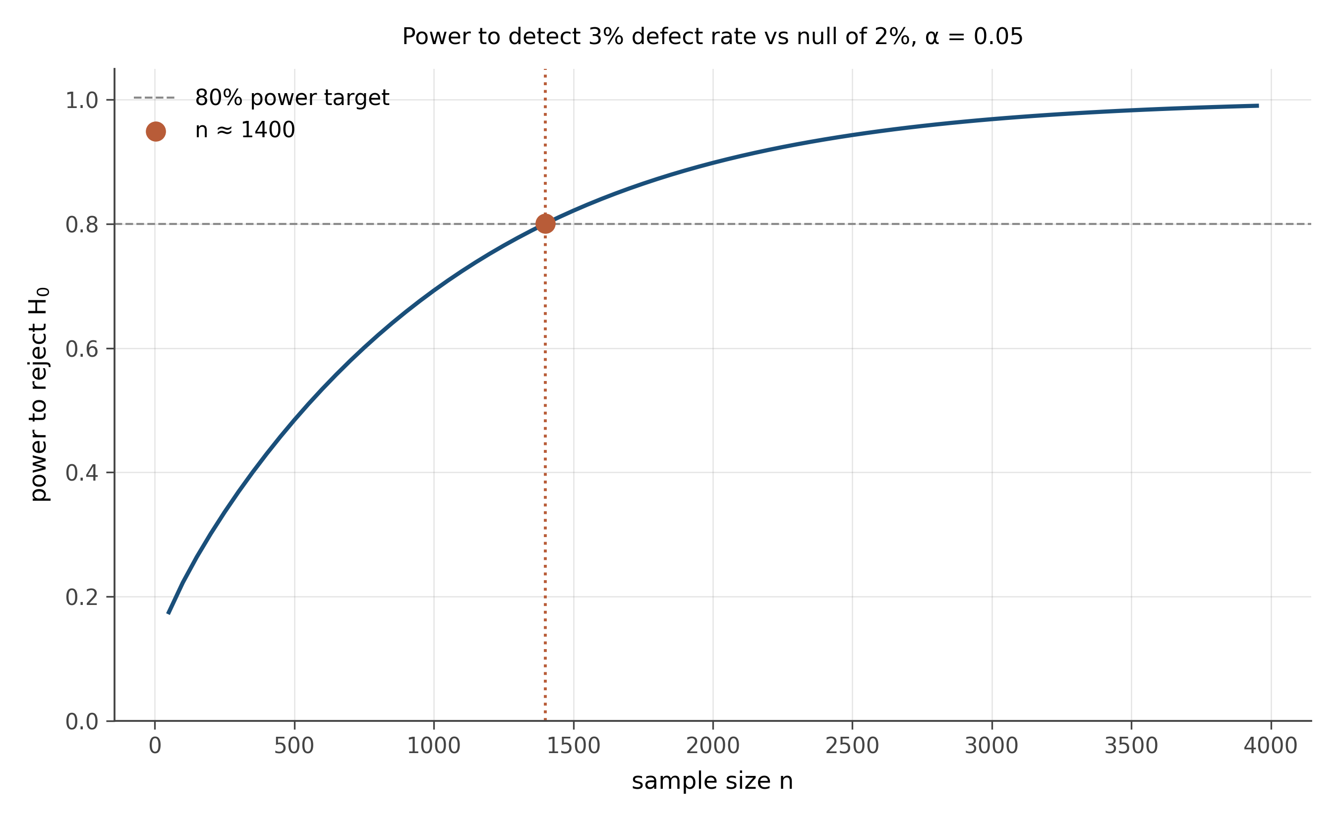
Setup. Detect p_1 = 0.03 vs p_0 = 0.02, one-sided, \alpha = 0.05, target power 1 - \beta = 0.80.
Approximate formula. For a one-sided proportion test at small p, the required sample size is approximately n \approx \frac{\left(z_{1-\alpha} \sqrt{p_0(1-p_0)} + z_{1-\beta} \sqrt{p_1(1-p_1)}\right)^2}{(p_1 - p_0)^2}. With z_{0.95} = 1.645 and z_{0.80} = 0.842: n \approx \frac{(1.645 \sqrt{0.0196} + 0.842 \sqrt{0.0291})^2}{0.0001} = \frac{(0.230 + 0.144)^2}{0.0001} \approx 1{,}400.
Interpretation. To have an 80% chance of detecting a true 3% defect rate when the null is 2%, you need to sample roughly 1,400 parts. The sample of 500 in problem 4 had power below 50% to detect this difference, which is why it failed to reject even though the empirical rate (2.8%) was above the threshold.
The general principle. Power scales with \sqrt{n}, with 1 / |\text{effect size}|, and with 1/\sqrt{p_0(1-p_0)}. Detecting smaller effects, or distinguishing rates near 0 or near 1, requires larger samples. Most underpowered studies fail to reject not because the null is true but because they were never going to be able to reject under any realistic alternative. Compute power before you collect data, not after.
16.7 Problem 7: Multiple testing
You run 100 independent hypothesis tests, each at \alpha = 0.05. None of the underlying nulls is actually false. How many of your tests do you expect to reject? What does this imply about reading published research?
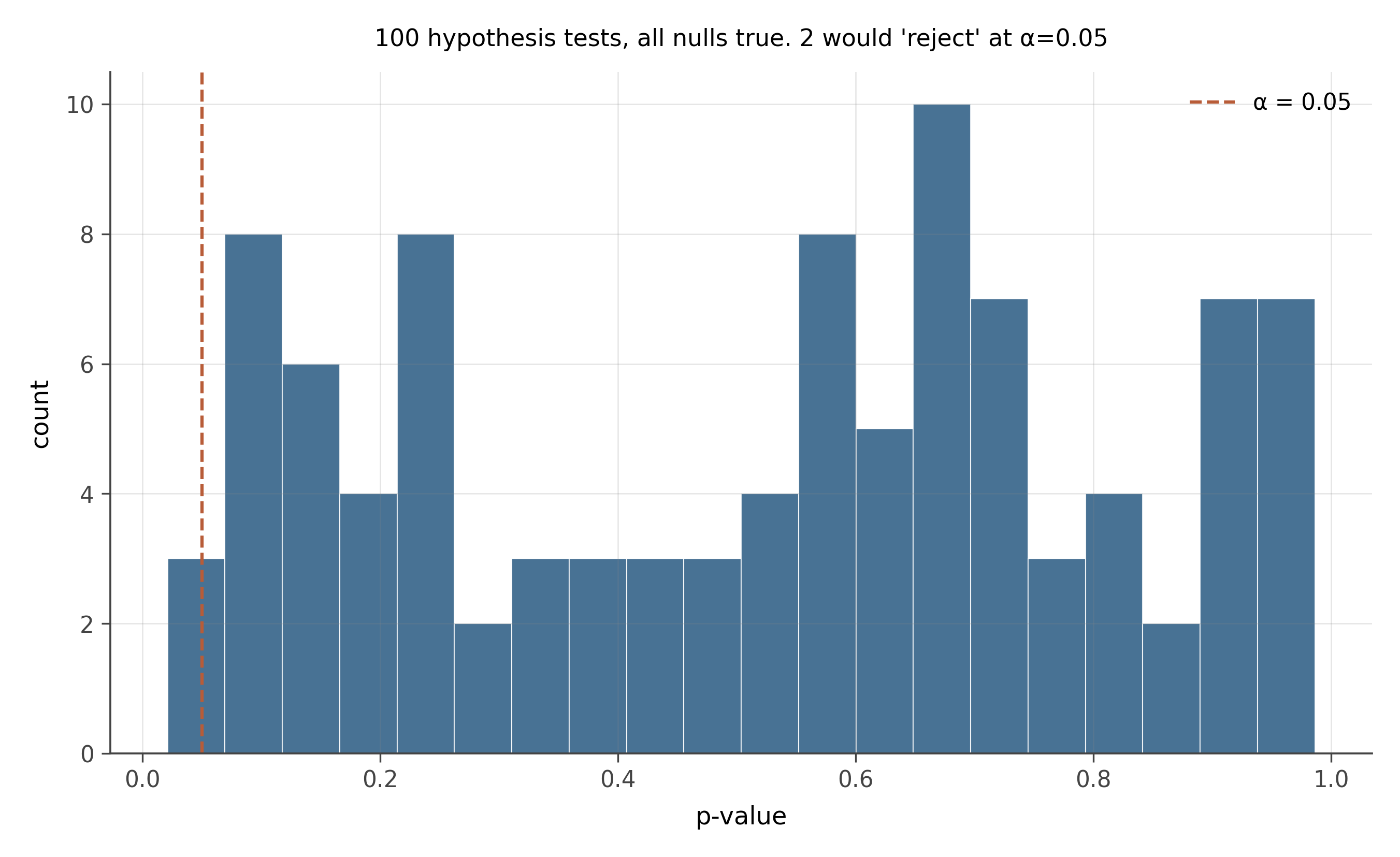
Expected rejections. Each test has probability 0.05 of rejecting under its (true) null, so expected number of rejections is 100 \cdot 0.05 = 5. The variance is 100 \cdot 0.05 \cdot 0.95 = 4.75, so the standard deviation is about 2.2. You should not be surprised to see anywhere from 0 to 10 false positives in 100 tests when every null is true.
Distribution of p-values. Under the null, each p-value is uniformly distributed on [0, 1]. The histogram of all 100 p-values should look approximately flat. The reason is direct: p is the cumulative probability under the null of seeing a statistic at least as extreme as the observed one, and the cumulative distribution of any continuous random variable is uniform when the variable is drawn from its true distribution.
Implication for reading research. A paper that reports 20 hypothesis tests and finds 3 significant at p < 0.05 has not necessarily found anything: the expected number of false positives at \alpha = 0.05 across 20 tests is one. Distinguishing real signal from chance requires either (a) pre-registration of the specific hypothesis being tested, or (b) multiple-testing correction. The two main correction methods are:
- Bonferroni: divide \alpha by the number of tests. With 20 tests, use \alpha = 0.0025 for each. Conservative but valid.
- Benjamini-Hochberg (FDR): controls the expected proportion of false positives among rejections rather than the family-wise error rate. Less conservative, more useful when many tests are run.
The replication crisis. A substantial fraction of published “significant” findings in psychology, biomedicine, and economics are false positives precisely because researchers ran many tests, reported only the significant ones, and did not correct for multiple comparisons. This is sometimes called p-hacking or the garden of forking paths. The defensive moves (pre-registration, full reporting of all tests run, mandatory FDR correction) are now standard in better journals and not yet standard everywhere else.
16.8 Problem 8: Effect size, not just significance
A study of 50,000 patients finds a “highly significant” association between coffee consumption and a small marker of inflammation. The reported p-value is 10^{-12}. The estimated effect is a 0.04% change in marker level per cup of coffee per day. Should you change your coffee habits?
The trap. A very small p-value with a huge sample does not mean the effect is large. With n = 50{,}000, the standard error of any estimate is tiny, so even a microscopically small effect will produce an enormous test statistic. The p-value tells you whether the effect is distinguishable from zero. It tells you nothing about whether the effect is meaningful.
The real question. Is 0.04% per cup a practically meaningful change in inflammation? Almost certainly not. Day-to-day variation in any biomarker is typically much larger than 0.04% from any single intervention. The signal is real (the data have ruled out exact zero) but it is so small that it disappears within ordinary noise.
Decision. No, do not change your coffee habits based on this study. The effect size is too small to matter for any individual.
The general lesson. Always report effect sizes alongside p-values. A standard formulation:
- “Coffee consumption was associated with a 0.04% increase in the inflammation marker per cup per day, 95% CI: (0.03%, 0.05%), p = 10^{-12}, n = 50{,}000. The effect is statistically distinguishable from zero but is small relative to typical day-to-day variation in this marker (approximately 5%) and unlikely to be clinically meaningful.”
This is the form every results paragraph should take. The journal-table convention of showing only stars and p-values systematically obscures effect sizes, which is one reason coefficient plots (chapter 8) are gradually replacing star-driven tables in modern research.
16.9 Real UK data
These three problems use two UK administrative datasets. The Scottish Index of Multiple Deprivation 2020 (SIMD 2020), published by the Scottish Government, scores all 6,976 Scottish data zones on multiple deprivation dimensions and assigns each a rank from 1 (most deprived) to 6,976 (least deprived). A data zone contains roughly 500–1,000 residents. The Land Registry Price Paid Data records every registered residential property transaction in England and Wales — a complete administrative record, not a sample.
16.9.1 Problem 9: Urban and rural deprivation in Scotland
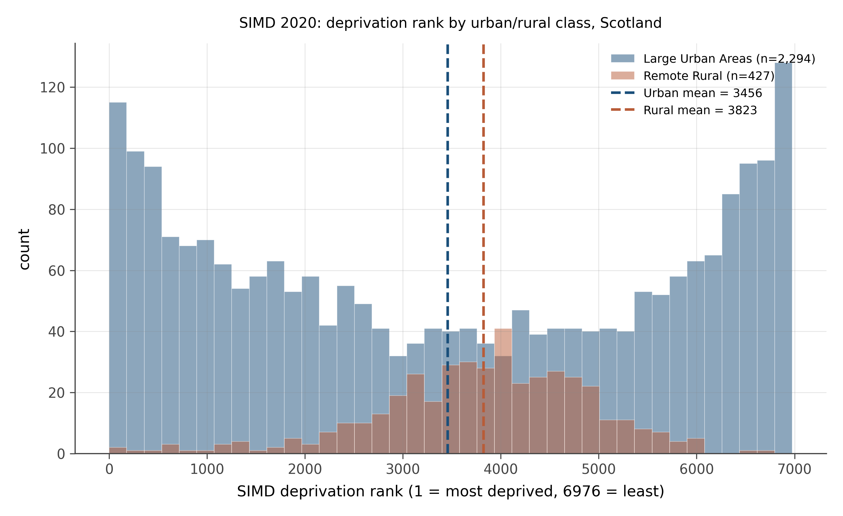
The SIMD assigns each data zone to an urban-rural class. Class 1 (Large Urban Areas) covers cities such as Glasgow, Edinburgh, Aberdeen, and Dundee. Class 6 (Remote Rural) covers sparsely populated areas more than a thirty-minute drive from a settlement of 10,000 people. The histogram below compares deprivation ranks across these two groups.
State and test the following hypothesis formally:
H_0: The mean deprivation rank is the same in Large Urban Areas and Remote Rural data zones. H_1: The two groups have different mean deprivation ranks.
- From the figure alone, which group appears more deprived on average? By roughly how much?
- What test is appropriate here? What assumptions does it require?
- The sample sizes are large. What does this imply for the power of the test?
- Suppose the test rejects at p < 0.001. A journalist writes: “Urban areas are significantly more deprived than rural ones.” Evaluate this claim carefully. Is it statistically justified? Is it practically informative?
Which group is more deprived? Large Urban Areas have lower mean ranks, meaning they are, on average, more deprived than Remote Rural areas. This may seem counterintuitive: rural poverty is real, but Scotland’s most severely deprived communities are concentrated in urban areas such as parts of Glasgow, Dundee, and Inverclyde. Remote Rural areas tend to cluster in the middle of the rank distribution, not at the deprived extreme.
Appropriate test. A two-sample t-test (Welch’s version, which does not assume equal variances). The assumptions are: (i) the two groups are independent samples of data zones, (ii) the ranks are approximately normally distributed within each group, or the sample sizes are large enough for the central limit theorem to apply. Both conditions are met here. The large sample sizes (hundreds to thousands of data zones per group) make the normality assumption largely irrelevant by CLT.
Power. Large sample sizes produce small standard errors, which means even modest differences in means will generate large test statistics and very small p-values. With hundreds of data zones in each group, the test has very high power to detect differences of even 100 rank positions.
Evaluating the journalist’s claim. “Statistically significant” (at p < 0.001) means the data rule out the null that the two groups have identical means, with high confidence. Whether this is “practically informative” is a separate question. The difference in mean ranks translates into a concrete difference in deprivation scores, and the researcher should report that difference alongside the p-value. The journalist’s framing is also slightly imprecise: urban areas as a whole are not “more deprived” than rural ones in a uniform sense. The urban distribution is more spread out — it contains Scotland’s most deprived and some of its least deprived zones. The rural distribution is narrower and centred higher. The claim is defensible in the sense of “lower mean rank for urban areas,” but the headline erases the within-group spread that is often as important as the difference in means.
16.9.2 Problem 10: London house prices versus the rest of England
A buyer’s group claims that London house prices are significantly higher than those in the rest of England. Using 2,000 randomly selected transactions from London and 2,000 from the rest of England (all from the Land Registry Price Paid Data, transactions below £2,000,000), test this claim at the 1% significance level.
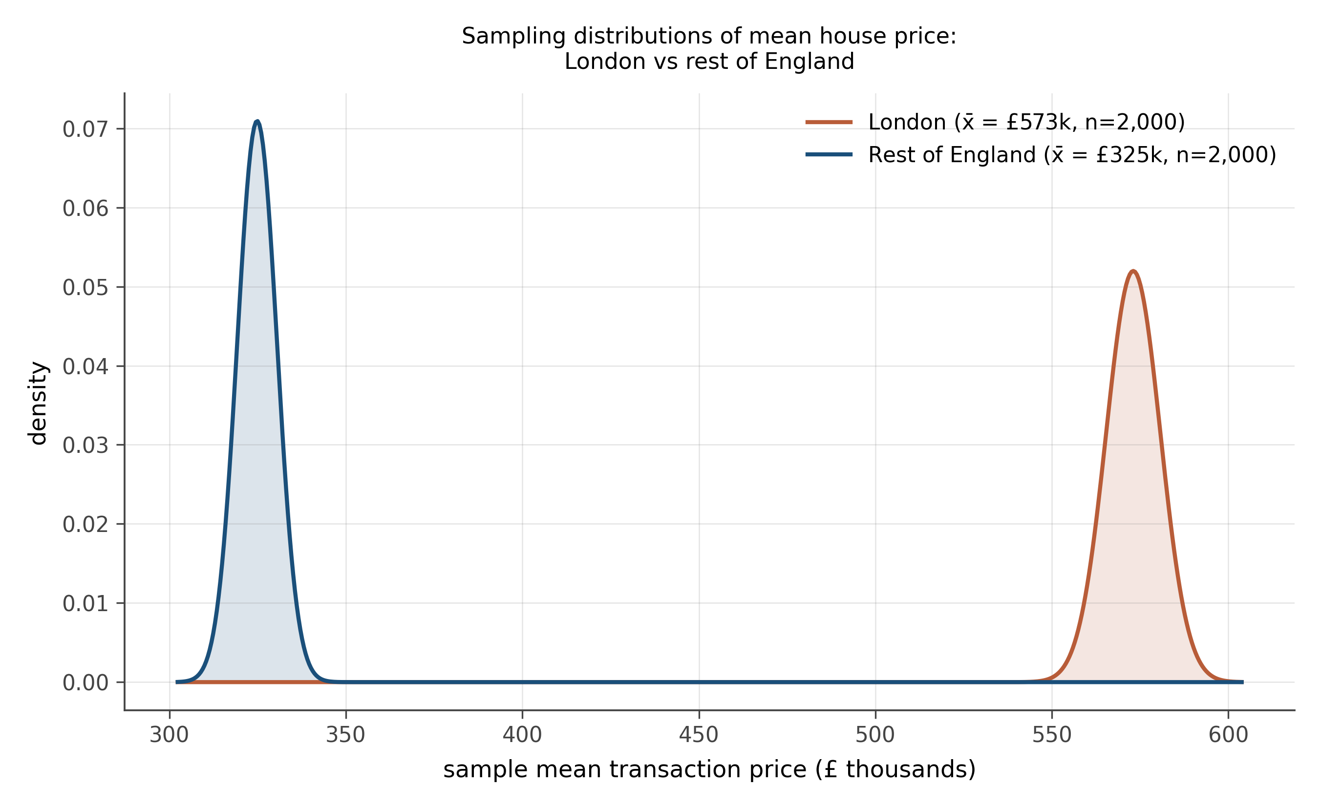
- From the figure, do the two sampling distributions overlap? What does the overlap (or lack of it) tell you before you compute any test statistic?
- Write out the null and alternative hypotheses formally.
- What kind of test is appropriate? Why not a paired t-test?
- The figure shows the sampling distributions of the two sample means, not the raw price distributions. Why does this distinction matter?
Overlap. The two sampling distributions are visibly separated, with little or no overlap. This is strong visual evidence against H_0 before any calculation. If the two population means were equal, we would expect the sampling distributions to be centred at the same value; they clearly are not.
Hypotheses. Let \mu_L and \mu_E denote the population mean transaction prices for London and the rest of England respectively.
H_0: \mu_L = \mu_E \qquad H_1: \mu_L > \mu_E
The claim is one-sided (London prices are higher), so a one-sided test at \alpha = 0.01 is appropriate, though a two-sided test at \alpha = 0.01 is also defensible if you want to account for the possibility of London prices being lower (which is implausible here but formally complete).
Test choice. A two-sample t-test (Welch’s). Not a paired test, because the London and rest-of-England transactions involve different properties and different buyers; there is no natural pairing. The two groups are independent random samples from different sub-populations of the market.
Sampling distribution vs raw distribution. The raw price distributions are heavily right-skewed (see workbook 1, problem 9). The sampling distributions of the sample means are approximately normal by the central limit theorem — even though individual prices are skewed, the average of 2,000 prices is very close to normally distributed. This is why the curves in the figure look like normal bells. The distinction matters because the t-test is applied to the means (which are approximately normal) not to the raw prices (which are not). With n = 2{,}000, the CLT approximation is excellent.
16.9.3 Problem 11: Are property types uniformly distributed?
The Land Registry records four main residential property types: Detached (D), Semi-detached (S), Terraced (T), and Flat/Maisonette (F). The bar chart below shows the observed counts in the dataset alongside what we would expect if all four types were equally common.
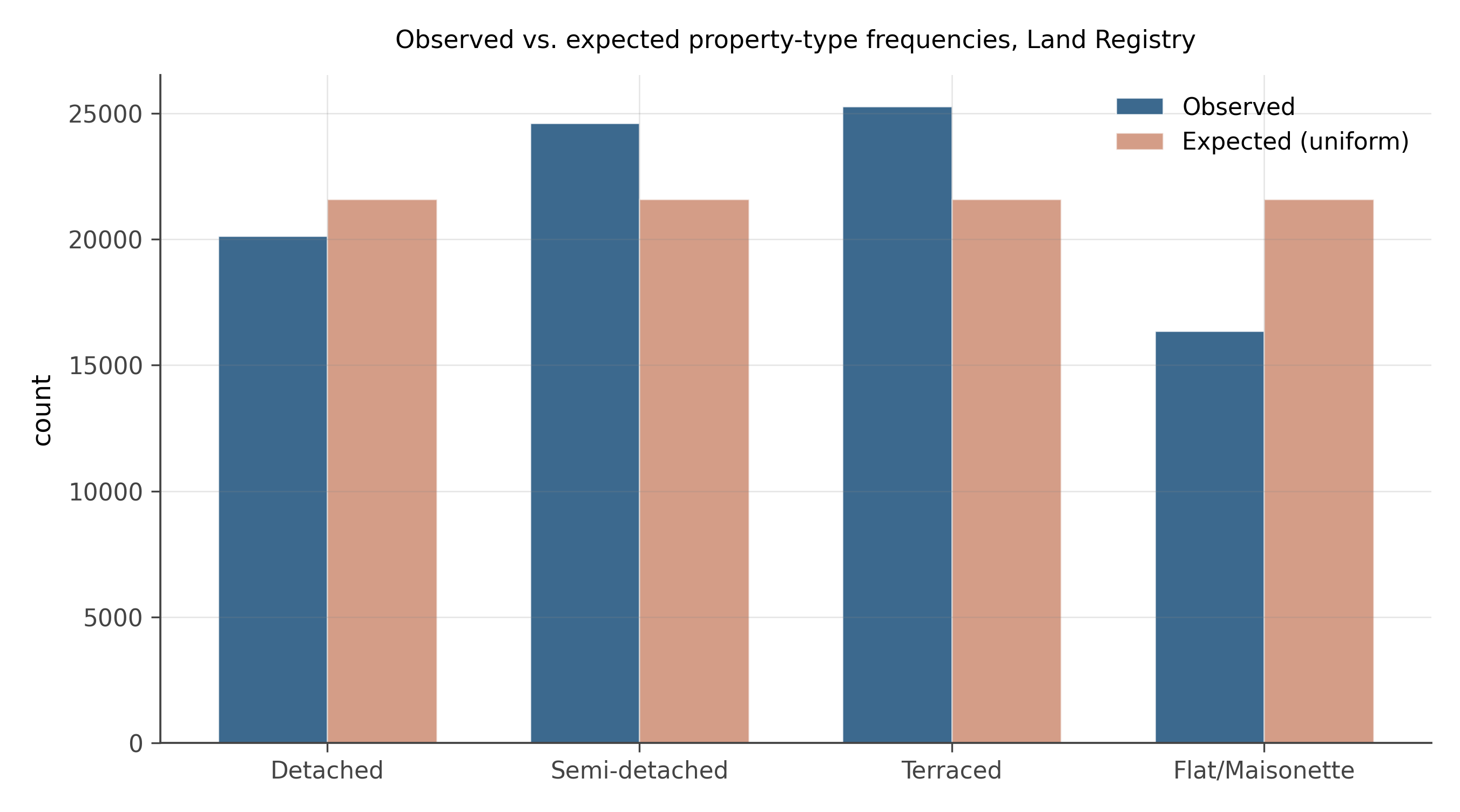
Test the null hypothesis that all four property types appear with equal frequency.
- From the figure, which property type is most over-represented relative to the uniform expectation? Which is most under-represented?
- State the null and alternative hypotheses for this test. What test statistic is appropriate?
- The chi-squared test statistic is \chi^2 = \sum (O_i - E_i)^2 / E_i. Compute it from the figure.
- With 3 degrees of freedom, the critical value at \alpha = 0.001 is approximately 16.3. What do you conclude?
Over/under-represented types. From the figure: Semi-detached and Terraced houses are the most common types, exceeding the uniform expectation. Detached houses are close to the uniform benchmark or slightly under. Flats and Maisonettes are substantially under-represented relative to what uniform proportions would predict.
Hypotheses. Let p_D, p_S, p_T, p_F denote the true proportions of each type.
H_0: p_D = p_S = p_T = p_F = 0.25 \qquad H_1: \text{at least one proportion differs}
The appropriate test is a chi-squared goodness-of-fit test. The test statistic is \chi^2 = \sum_{i=1}^{4} (O_i - E_i)^2 / E_i, where O_i are observed counts and E_i = n/4 for each category.
Computing \chi^2. The exact values depend on the counts in the dataset. With roughly 93,000 transactions and a clear visual departure from uniformity, the chi-squared statistic will be very large. Even a 2% departure from 25% in one cell contributes roughly (0.02 \times 93000)^2 / (0.25 \times 93000) \approx 1{,}550 to the statistic. The total \chi^2 will be orders of magnitude above any standard critical value.
Conclusion. The null of uniform proportions is emphatically rejected. Property types are not equally distributed in the Land Registry: semi-detached and terraced houses dominate because they are the dominant building stock of Britain’s post-war suburban expansion. Detached houses are rarer because they require more land. Flats, while numerous in absolute terms, make up a smaller share of total transactions partly because more flats are rented rather than sold. Rejecting the uniform null is not surprising — it is the baseline anyone familiar with British housing stock would predict. This problem illustrates a recurring issue with large datasets: with 93,000 observations, the test has overwhelming power and will reject almost any null hypothesis, including ones that are only trivially wrong. Statistical significance does not imply economic or policy significance; the practical question is whether the departures from uniformity are large enough to matter for whatever decision you are making.
16.10 What you practiced
The five-part structure is the scaffold:
- State H_0 and H_1.
- Pick the test.
- Compute the statistic.
- Compute the p-value.
- Decide, and report the effect size and its uncertainty.
The most important takeaways from the eight problems:
- Different questions need different tests. Match the data structure to the test, not the test to your habit.
- A p-value is conditional on H_0 being true. It is not the probability that the null is true, and not the probability the result will replicate.
- Statistical significance is not practical significance. With enough data, you can detect arbitrarily small effects. Always report the effect size.
- Failing to reject is not the same as accepting. It usually means the sample is too small.
- Power matters. Compute it before collecting data. An underpowered study cannot tell you anything about real effects.
- Multiple testing inflates false positives. Ten tests at \alpha = 0.05 are expected to produce roughly half a false positive even when every null is true. Twenty tests, one false positive. Correct for this or pre-register your hypotheses.
Real applied work in Parts II and III runs these tests inside regressions, in causal-inference designs, with clustered standard errors, and across many specifications. The mechanics are the same; the chains of reasoning get longer. This workbook is the foundation everything else stands on.