12 Reading equations
- The three-layer vocabulary of mathematical notation
- How to read aloud: conditional expectation, OLS in matrix form, Bayes’ theorem
- Translation drills, English-to-math and math-to-English
12.1 Equations are sentences
Most students approach equations with a particular kind of dread. The dread comes from a specific misconception: that an equation is something you compute with, not something you read. The book has been claiming since the preface that this is wrong. This chapter is where the claim becomes operational.
An equation is a sentence in a language. It has a subject. It has a predicate. It has modifiers, conjunctions, and rhetorical moves. Reading an equation well is the same kind of skill as reading a paragraph well, and it can be taught the same way: by parsing the parts, by drilling translation between languages, and by reading aloud often enough that the second language becomes natural.
The chapter has three parts. First, the alphabet and grammar of mathematical notation: what each kind of symbol does and which conventions get used. Second, three worked-example expressions parsed in detail (a conditional expectation, the OLS estimator, Bayes’ theorem). Third, a translation drill in both directions, with answers.
When you finish this chapter, you will not know any new math. You will read math you have already seen with substantially less friction.
12.2 The vocabulary
A piece of mathematical notation has three layers, the same three layers a sentence in English has.
Symbols. The atoms. Letters from the Latin and Greek alphabets, operators (+, −, ×, ÷, \sum, \prod, \int), relations (=, <, >, ≤, ≥, ≠, ≈, \propto), grouping symbols (parens, brackets, braces). Each symbol has a primary meaning and sometimes a context-specific one. The summation sign \sum always means “add up the things on the right of me, indexed by the variable below me.” That is its meaning, full stop.
Conventions. Implicit rules about which symbols mean what. Greek letters typically denote population parameters: the unknown true values you would know if you had infinite data. Roman letters typically denote estimates or sample quantities. A hat over a Roman letter, \hat\beta, marks an estimator: a function of the data that targets some unknown parameter. Bold letters (\bm{x}, \bm{X}) denote vectors and matrices. Subscripts mark indices (x_i is the i-th observation; \beta_1 is the first coefficient). These are conventions, not laws, but the same conventions are used by virtually every statistics and econometrics textbook, and once you know them, equations become much easier to read.
Compositional rules. How symbols and conventions assemble into expressions. Function application, f(x), means “apply function f to argument x.” Conditional notation, Y \mid X, means “the random variable Y, given that we condition on X.” Probability and expectation are operators that take a random variable as their argument. The same rules apply at every level of nesting, which is why a complex expression can be parsed by working from the inside out.
These three layers are the entire language. Everything from chapter 1 onward will use them. Knowing them makes reading the rest of the book a different experience.
12.3 Three expressions, parsed aloud
The best way to learn a language is to read it. Three expressions follow, each with a parsing pass: what each piece does, how it combines, and how the whole expression is read aloud. After the third one, the rest of the book’s notation should feel less foreign.
12.3.1 Expression 1: \E[Y \mid X = x]
Read aloud: the expected value of Y given that X equals x.
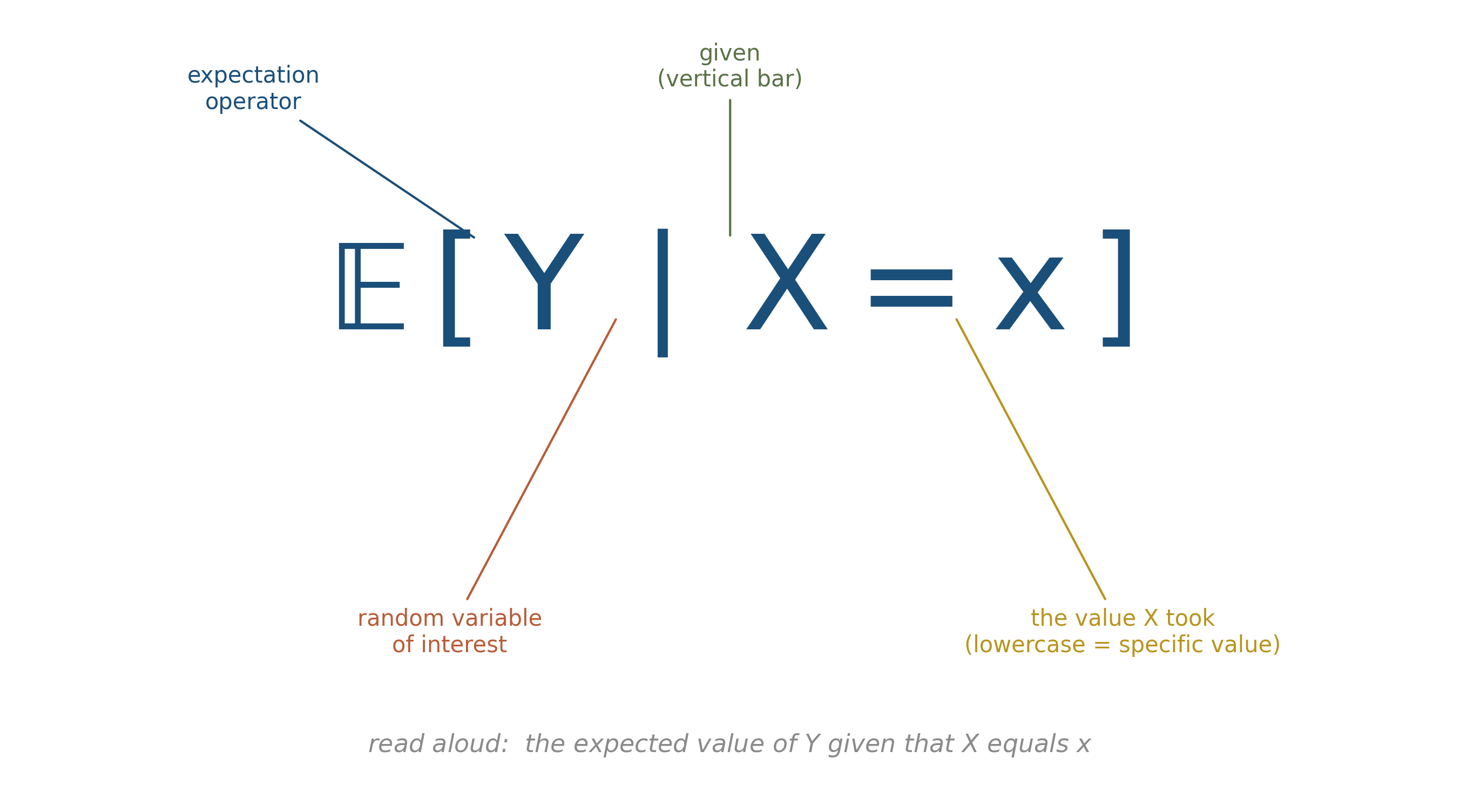
Layer by layer:
- Y is a random variable. We do not yet know its value, but it has a distribution.
- X = x is a conditioning event. The capital X is also a random variable; the lowercase x is a specific value of it. The expression X = x is the event “X took the value x.”
- The vertical bar \mid means “given.” It separates the thing being asked about (left) from the conditioning information (right).
- The brackets [\cdot] denote that what is inside is the argument of the operator \E.
- \E is the expectation operator. It takes a random variable (or a function of one) as its argument and returns a number: the average over the distribution of that random variable.
The whole expression returns a number: the average value of Y over the conditional distribution of Y given that X takes the value x.
Where you have already seen this. In chapter 2, when we conditioned on hearts and asked about the probability of a face card, we were computing P(\text{face} \mid \text{heart}). The same operation, with probability instead of expectation, lives inside \E[Y \mid X = x] when Y is binary.
12.3.2 Expression 2: \hat\beta = (\bm{X}^\top\bm{X})^{-1}\bm{X}^\top\bm{y}
Read aloud: beta-hat equals X-transpose-X inverse, times X-transpose-y.
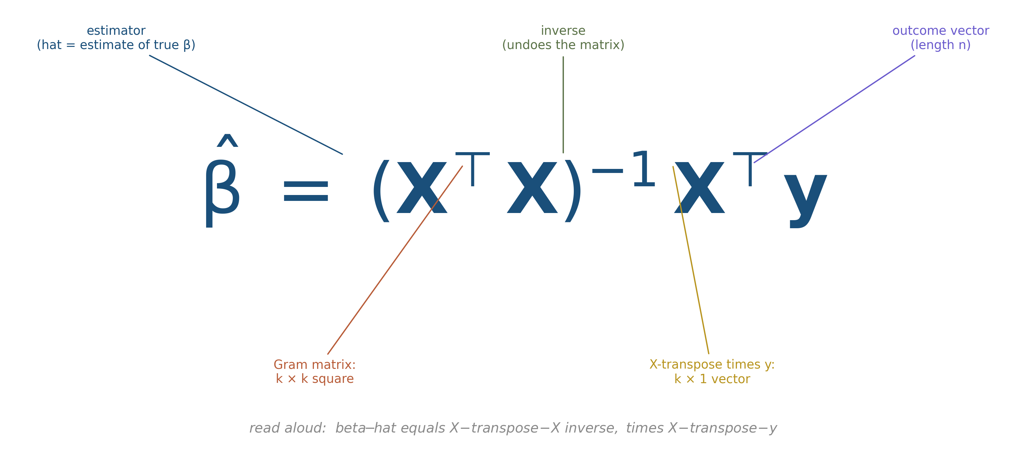
This is the OLS regression estimator in matrix form. It looks scary. The pieces are not.
- \hat\beta is the estimator: a vector of estimated coefficients. The hat marks it as an estimate of the unknown true \beta.
- \bm{X} is the design matrix: a rectangular array with one row per observation and one column per regressor. Its dimensions are n rows by k columns, where n is the sample size and k is the number of regressors.
- \bm{X}^\top is the transpose of \bm{X}. The rows become columns and vice versa, so its dimensions are k by n.
- \bm{X}^\top\bm{X} is a k by k matrix: the result of multiplying transpose-X by X. Sometimes called the Gram matrix of \bm{X}.
- (\bm{X}^\top\bm{X})^{-1} is the inverse of that matrix. The inverse exists when the columns of \bm{X} are linearly independent (no perfect collinearity).
- \bm{y} is the vector of outcomes, length n.
- \bm{X}^\top\bm{y} is the result of multiplying transpose-X by the outcome vector: a vector of length k.
Putting it together. The estimator \hat\beta is computed by inverting one k \times k matrix and multiplying it by one k \times 1 vector. In one dimension, when k = 1 and \bm{X} is a single column of x-values, the formula reduces to \hat\beta = \sum x_i y_i / \sum x_i^2, which is the textbook formula for a slope through the origin. The matrix form is the same calculation, generalized to many predictors at once.
We will derive this expression carefully in chapter 24. For now, the goal is to look at it without flinching.
12.3.3 Expression 3: P(A \mid B) = \dfrac{P(B \mid A) \, P(A)}{P(B)}
Read aloud: the probability of A given B equals the probability of B given A, times the probability of A, divided by the probability of B.
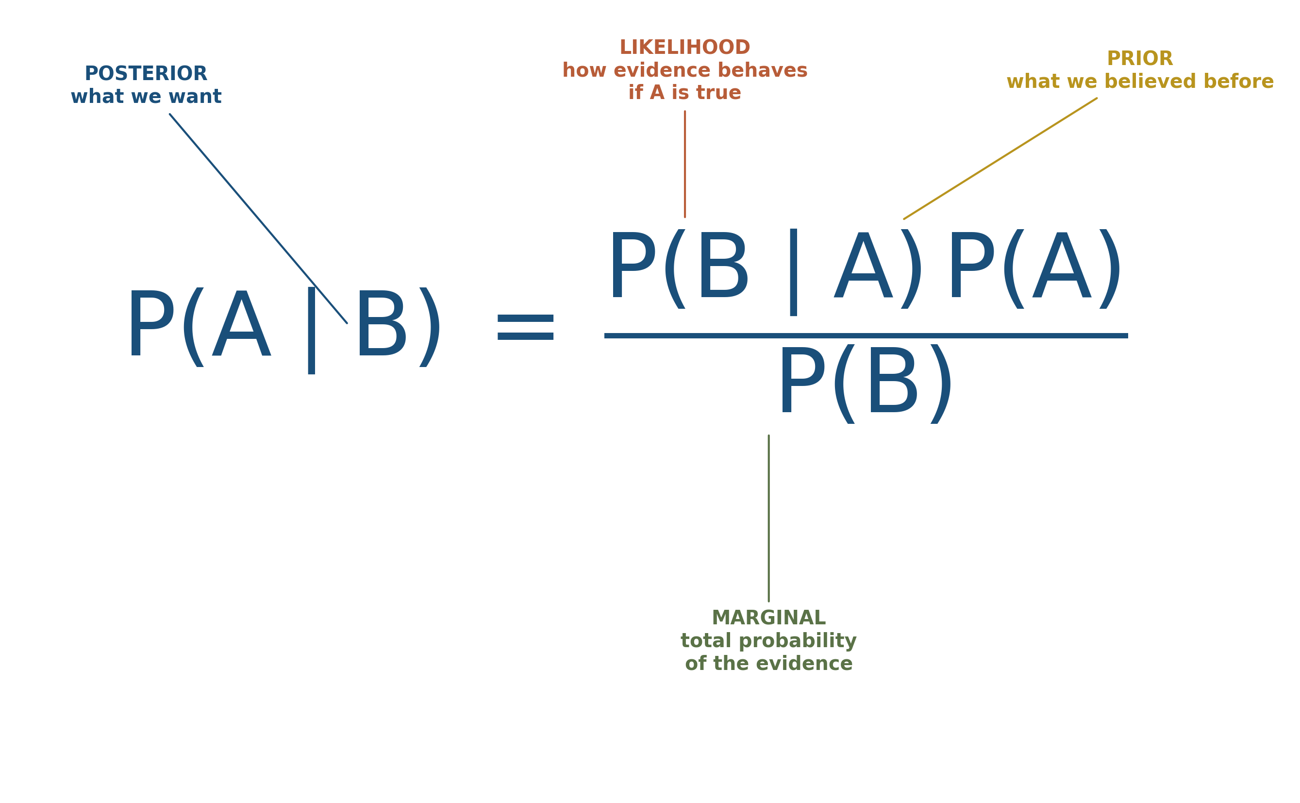
This is Bayes’ theorem, which we met visually in chapter 2 with the disease-test grid. The expression compresses the entire grid into a formula.
- P(A \mid B) is the posterior: what we want to know.
- P(B \mid A) is the likelihood: how the evidence behaves if A is true.
- P(A) is the prior: what we believed before the evidence.
- P(B) is the marginal: the total probability of the evidence, often computed as P(B \mid A)P(A) + P(B \mid \neg A)P(\neg A).
The formula is the rectangle picture you already know. Its numerator is the size of the upper-left tile (sick and positive). Its denominator is the size of the entire positive column (sick-and-positive plus well-and-positive). Their ratio is the conditional probability.
When you encounter Bayes in any later chapter, picture the grid first and translate the formula into rectangles second. The picture is more honest, and the formula is the picture written down.
12.4 Translation drill: English to math
Translate each English statement into a mathematical expression. Answers in the next subsection.
- The probability that a randomly chosen observation has X greater than 5.
- The expected value of Y, conditional on X being equal to 3.
- The variance of the sum of two independent random variables.
- The estimator \hat\theta that maximizes the likelihood function L(\theta).
- A vector of n ones.
Possible answers:
- P(X > 5)
- \E[Y \mid X = 3]
- \Var(X + Y) = \Var(X) + \Var(Y) when X and Y are independent
- \hat\theta = \arg\max_\theta L(\theta)
- \bm{1}_n
12.5 Translation drill: math to English
Translate each expression into English a senator could understand without lying.
- \hat\mu = \frac{1}{n}\sum_{i=1}^{n} x_i
- \Var(\hat\mu) = \sigma^2 / n
- H_0: \beta = 0
- \E[\hat\beta] = \beta
- \hat\beta \pm 1.96 \cdot \text{SE}(\hat\beta)
Possible answers (English versions, not the only correct ones):
- The estimated mean is the average of the observed values.
- The variance of the sample mean shrinks like one over n: more data gives a more precise estimate, in a way that is square-root-of-n.
- The null hypothesis says the coefficient is zero.
- The estimator is unbiased: on average across many samples, it equals the true value.
- A 95% confidence interval for the coefficient is the point estimate plus or minus about two standard errors.
Reading aloud is the trick. A statistician hears these sentences in their head when they look at the symbols. After enough drilling, you will too.
Equations are sentences in a language. They have subjects, predicates, and modifiers, and they parse from the inside out. The vocabulary is small (a few dozen symbols, a few dozen conventions, a small set of compositional rules). Reading them aloud is not metaphorical; it is the literal practice that makes them feel like sentences. This chapter is the keystone of the book: every later chapter assumes you can do what was just demonstrated.
Open any chapter you have finished and find an equation you previously skipped past. Parse it now using the three-layer approach: identify each symbol, identify the conventions in play, and parse the composition from the inside out. Read the result aloud.
Then write the same expression as a sentence in English, the way you would say it to a colleague who had never seen the notation.
Repeat with two more equations from later in the book. The skill compounds quickly.
This chapter described the conventions used in this book and in most of mathematical statistics: Greek for parameters, Roman with hats for estimators, bold for vectors and matrices, \E for expectation, P for probability, \sum for summation. These conventions are not universal.
Engineering uses different conventions. Physics uses different conventions. Some economists use \bar{x} where statisticians would use \hat\mu. Some Bayesians use p(\theta \mid y) where frequentists would use f_{\theta \mid Y}(\theta \mid y). The conventions of measure theory diverge from the conventions of probability theory in subtle ways.
The best defense against notation confusion is to read the first appearance of any symbol carefully and not assume it means what the same symbol meant in another paper. Authors who care about their readers parse their notation explicitly the first time they introduce it. Authors who do not are not the authors you want to spend time on.
The chapter argued that reading equations is a learnable skill, not a talent. Where in your own life have you treated math as inaccessible because nobody explained the parsing? What changed when somebody finally did?
Translation drills work because they force production, not just consumption. Pick one expression you parsed in this chapter and write it three different ways in English. Which is most precise? Which would you actually use in a memo?
The conventions are not universal but they are widely shared. Why might a field’s choice of notation reflect its priorities? What does it tell you that econometrics borrows so much from probability theory and so little from physics?
The pedagogical work of teaching mathematical notation as a language is recent and remains contested. McElreath’s Statistical Rethinking, Cunningham’s Mixtape, and a small number of other textbooks have moved in this direction: parsing equations explicitly, drilling translation, refusing the convention that notation should be installed without comment.
The traditional alternative, what most graduate textbooks still do, is to assume the reader can already read the notation and to use it without translation. This works for readers who came up through a long apprenticeship in mathematical writing. It excludes everyone else.
The current frontier is in mathematical-writing pedagogy specifically: how to teach notation as a craft, alongside the substance it encodes. Knuth’s Mathematical Writing and Halmos’s classic essay “How to Write Mathematics” are the foundations. The newer literature builds on them.
12.6 Practice problems
Read aloud, in your own words: P(X = x \mid Y = y).
Parse each piece of \hat\sigma^2 = \frac{1}{n-1} \sum_{i=1}^n (x_i - \bar{x})^2. Identify the hat, the subscript, the summation, the sample mean, the squared deviation, and the n-1.
Translate to math: “The probability that the absolute difference between the sample mean and the population mean exceeds two standard errors.”
Translate to English: \E[X^2] = \Var(X) + \E[X]^2.
Pick an equation from any paper in your field. Parse it using the three-layer approach. Write the English translation as a sentence you would say aloud.
Looking ahead
Chapter 10: Reading tables. Chapter 9 taught you to read equations. The next chapter does the same for tables, which are the other primary way working researchers compress quantitative arguments into a small printable area. Continue →