4 Numbers on the page
- How to read a dataset before you analyze it
- The four kinds of variable and what arithmetic each one supports
- The eight-question audit to run on every new dataset
4.1 What you just did
Here is a small piece of a real-shaped dataset: bilateral trade flows for six countries observed over a decade, one row per pair-of-countries per year. Look at it for ten seconds before reading on.
| year | exporter | importer | exports (USD millions) | exporter GDP (USD T) | importer GDP (USD T) | distance (km) | common language | common border |
|---|---|---|---|---|---|---|---|---|
| 2023 | USA | CHN | 85,058 | 27.36 | 17.79 | 11,587 | 0 | 0 |
| 2023 | USA | DEU | 28,039 | 27.36 | 4.46 | 7,850 | 0 | 0 |
| 2023 | USA | JPN | 27,112 | 27.36 | 4.21 | 9,997 | 0 | 0 |
| 2023 | USA | GBR | 34,137 | 27.36 | 3.34 | 6,979 | 1 | 0 |
| 2023 | USA | KOR | 9,602 | 27.36 | 1.71 | 10,534 | 0 | 0 |
| 2023 | CHN | USA | 145,847 | 17.79 | 27.36 | 11,587 | 0 | 0 |
Ten seconds. What did your eye do?
It found the rows and the columns. It noticed each row contained the same kinds of things in the same order. It registered that some columns held names (USA, CHN, DEU) and some held numbers, and that the numbers came in different magnitudes. It parsed “85,058” as eighty-five thousand of something, possibly more if you bothered to figure out the units, possibly the size of an entire country’s exports to another country in a year. You probably started asking questions. Why does China export almost twice as much to the United States as the United States exports back? Why does the US export more to the much smaller economies of Germany and Japan than to Korea? What does “common language” mean as a number rather than as a word, and why is it 1 for the US-UK row and 0 for everyone else?
Nobody taught you to do any of that. You just did it.
This book is about the difference between doing it instinctively and doing it deliberately. Most people who say they are bad at math, or at any of the disciplines that wear quantitative clothes, are not bad at the seeing. They are bad at the next step, the one where what your eye noticed gets written down precisely enough to argue with. Here is the claim the rest of this book will try to demonstrate: the gap between those two skills is much smaller than it looks, and bridging it does not require you to become a different kind of person. You already do most of the work. We are going to slow down and notice how.
Chapter 1 is the easiest one. It establishes a single fact about almost every dataset you will ever meet, that data is rectangular and the rectangle is not a notational accident, and then catalogs the kinds of things that can live in a column. By the end of this chapter you will have a vocabulary for talking about any dataset, the way you already have one for talking about a paragraph of text. The vocabulary lets you decompose a dataset into parts, ask what each part is doing, and figure out which questions are worth asking before any analysis happens. The trade slice on this page is going to be a recurring character. By chapter five you will know it as well as you know your own kitchen.
A note on how to read this book before we start. You can read at three depths. The narrative goes straight through and requires no math beyond what came before. If you want the math, the technical sections develop it properly without interrupting the narrative. At the end of every chapter, a short frontier note points at what current research is fighting about. Pick the depths that suit you, and come back for the others later.
One more thing. When you encounter an equation, read it aloud. Out loud. Even if you do not yet know what every symbol means. Equations are sentences with a subject, a verb, and modifiers, and pretending they are not is the single biggest mistake students make in their first statistics course. We are going to fix that one immediately.
4.2 The shape
Every dataset you will ever look at is a rectangle. Some rectangles are tiny, two rows by three columns. Some are vast, millions of rows by hundreds of columns. The rule is the same at any size. Each row is one thing being observed. Each column is one thing being measured about it.
In our trade slice, every row is one country’s exports to one other country in one specific year. The first row, USA to CHN in 2023, is one observation. Just one. The next row is a different observation, USA to DEU in 2023, with its own values for everything. The columns describe the attributes you can attach to a row: the year, the exporter, the importer, the dollar value of exports, the GDP of each side, the great-circle distance between them, whether they share a language, whether they share a border.
This sounds obvious. It is not. The first question to ask of any dataset, before any analysis, is: what is one row? Until you answer that, you cannot do anything correctly with the data, because the same numbers can mean wildly different things depending on what the row represents.
Take our slice. One row is one country-pair-year. Three hundred rows total, six countries with five trading partners each over ten years. Suppose we instead aggregated to one-country-year. We would have sixty rows (six countries times ten years), and “exports” would mean each country’s total exports to the world rather than to a specific partner. Aggregate further to one-country and we would have six rows. Summarize to one-year and we would have ten. Same underlying facts, four different shapes, four different statistical worlds.
The unit of analysis is not a notational detail. It is a substantive choice that decides everything downstream. A regression run on country-year data answers different questions than a regression run on dyad-year data, and the same coefficient labeled “the effect of distance on trade” means almost incomparable things in the two settings. When you read a paper, the first thing to figure out is what one row of their dataset is. When you write your own analysis, the first thing to decide is what you want one row to be.
A column, on the other hand, is one variable measured across all the rows. The “distance_km” column has the same definition in every row, namely how far apart the two countries are. In our slice that number is the same every time the same pair appears, which is itself a clue about the data. Distance does not depend on the year. It is redundant across the time dimension. (We will come back to that. It matters for how regression standard errors should behave when observations within a country-pair are correlated, which they are.)
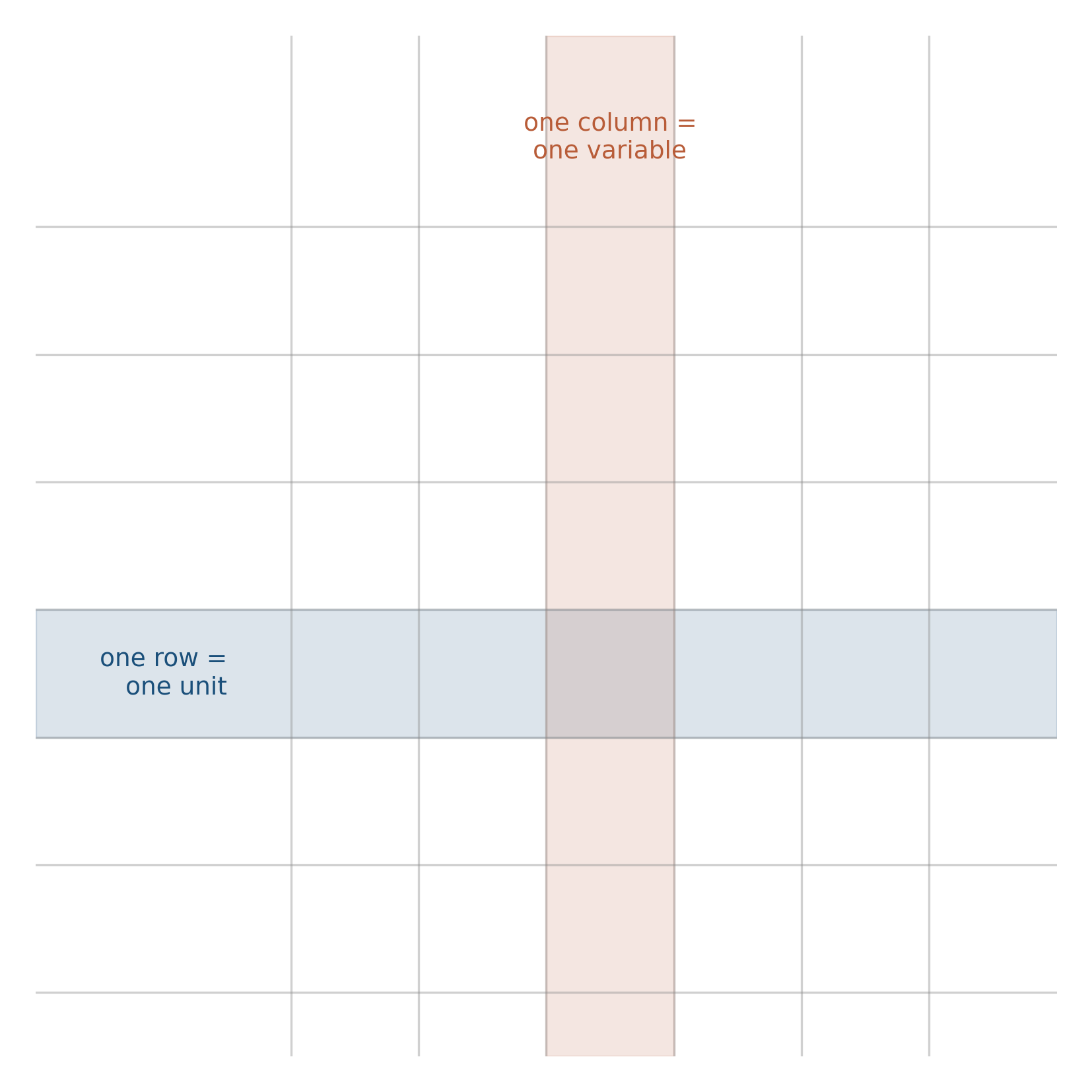
Burn this image into your visual cortex now. You will need it for the rest of the book. Whatever you are looking at, however many variables and however many observations, the rectangle is the underlying shape. The skill the book teaches is what to do once you see it.
4.3 What lives in a column
Columns come in flavors. The flavor matters because it determines what arithmetic the column will support.
The simplest distinction is between columns of numbers and columns of labels. Dollar value of exports: number. Country code USA: label. You can take the average of a number column and have it mean something. You cannot take the average of a column of country codes; the “average country” between USA and DEU is not a sensible thing. The exports-weighted average distance between trade partners, by contrast, is a real quantity that some people compute on purpose.
Statisticians divide variables into four flavors, and the difference between them comes down to what operations the values support.
Categorical, unordered (nominal). The values are names with no built-in ranking: country codes, sex, eye color, whether someone owns a passport. The only sensible operations are counting how often each value appears and asking whether two rows share the same value. USA and DEU are different. There is no answer to “is USA bigger than DEU.”
Categorical, ordered (ordinal). Order matters, but the gaps between adjacent values do not. Education levels (high school, college, graduate). Survey responses from strongly-disagree to strongly-agree. Movie ratings out of five. The difference between “agree” and “strongly agree” is not necessarily the same size as the difference between “neutral” and “agree.” You can sort the values. You can talk about medians. Treating the numbers as if they were dollars and computing an average is a substantive choice that needs defending in print.
S. S. Stevens (1946) is the canonical reference for the four levels of measurement (nominal, ordinal, interval, ratio). The four-flavor split here is the working consensus in modern applied work; some methodologists argue for finer or coarser distinctions, none has stuck.
Quantitative, discrete. Counts of things. The number of children in a household, the number of trade partners a country has in a given year. The values are real numbers and arithmetic works, but the values can only be whole numbers. You cannot have 2.4 children. The Poisson distribution, which we will meet in chapter three, is the natural home of this kind of variable.
Quantitative, continuous. Dollars, distances, time intervals, temperatures. Arithmetic works fully. The exports column in our slice is continuous, and so is GDP, and so is distance.
A common trap, especially when you are reading other people’s data: things that look like numbers and aren’t. ZIP codes. Phone numbers. Survey response IDs. The numeric country code 840 used for the United States in some bilateral databases. These are stored as integers, and a careless analyst will compute the mean ZIP code of a sample, get a result that is mathematically valid and substantively meaningless, and not notice. The number is a label that happens to look like a number. The statistical operation has to match what the column actually represents, not what its storage type happens to be.
Now the opposite trap: things that don’t look like numbers and are. Yes/no answers, encoded as 0 and 1. Dummy variables for whether a row meets some condition. The “common_language” column in our slice is one of these. It is a yes/no, encoded as 0 or 1, and you can absolutely compute its average. The mean of a 0/1 column is the proportion of rows where the value is 1. We use this constantly.
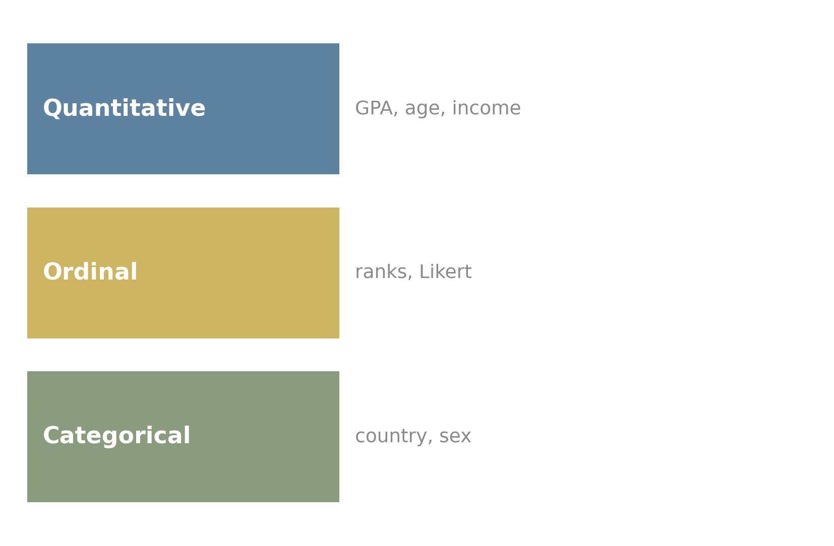
You will spend more of your statistical life than you would guess just figuring out what kind of variable each column is. It is the foundation for everything that follows, and it is almost never written down explicitly in the dataset itself. Doing it carefully is one of the easy wins of getting good at this.
4.4 First questions
Every time you sit down with a new dataset, before any analysis, run a short list of questions through your head. The list takes ten minutes for a small dataset and an afternoon for a serious one. It is the difference between an analysis you can defend and an analysis that quietly breaks underneath you.
Eight questions. Memorize the list.
1. What is one row? We did this already. Until you can name the unit of analysis without thinking, you cannot do anything else correctly. In our trade slice, one row is one country-pair-year.
2. How many rows, how many columns? For our slice, 300 rows and 9 columns. This sounds like trivia. It is not. The shape sets the cost of mistakes. With 300 rows you can eyeball almost anything; with 300 million you cannot. You will adopt different tools, do different sanity checks, and worry about different things as the row count grows.
3. What is the type of each column? Number or label. If number, continuous or discrete. If label, ordered or unordered. Walk every column. Be specific about borderline cases (the common_language column is technically categorical but encoded as 0/1 so you can average it, and you will).
4. What are the units? “Exports” is meaningless without “USD millions, current prices.” “Distance” needs “kilometers.” “GDP” needs “trillions of USD” and ideally “nominal vs. real, base year.” A staggering fraction of bad analyses come from someone forgetting that the units in two columns don’t match. The codebook in data/trade/codebook.md is the source of truth for our slice. Read it.
5. What is the time period? What is the geographic scope? Our slice covers 2014 to 2023, six countries chosen for size and student recognizability. Limited. A real bilateral trade panel covers 200 territories and goes back decades. Whatever your slice is, the scope is part of every claim you can make.
6. Where did the data come from, and what survived the journey? Raw data is messy. Clean data is the result of decisions: which observations to drop, which variables to re-code, which missing values to impute, which outliers to keep or remove. Every one of those decisions is a place where signal can leak. The processing script is part of the data. So is the person who wrote it.
7. What is missing? The thing the dataset doesn’t have is often more important than the thing it does. Our slice has six countries. Missing: every country except those six, every year before 2014, every product category, every direction of investment. Any conclusion drawn from this slice is conditional on those exclusions. A good analyst names the absences before drawing the inferences.
8. What looks weird? Look at the data. Sort by exports, find the smallest and largest values, check whether they make sense. Look at the distance column, find the row where two countries are improbably close or far, ask why. Look at the GDP columns, look for off-by-1000 unit confusion. The first ten minutes of weirdness-hunting saves the next ten hours.
These eight questions will not catch every problem. They will catch most. Run them every time. The discipline is what separates analysis from rationalization.
The rectangular structure described in this chapter is one specific arrangement called tidy data, formalized by Wickham (2014). A dataset is tidy when:
- Each variable forms a column.
- Each observation forms a row.
- Each type of observational unit forms a table.
These three conditions are equivalent to a special kind of relational normal form. The first two are the rectangular structure we have been discussing. The third is the rule that distinct kinds of things (countries, country-pairs, years) live in distinct tables, joined by keys, rather than crammed into a single table with mixed grain.
Many real datasets are not tidy. Wide-format panels, wide-format surveys, and aggregated tables encountered in the wild often fail one or more conditions. Most data analysis begins with tidying: reshaping data into the rectangular form. Most data analysis errors begin with someone forgetting which form they are in.
The reference is Hadley Wickham, “Tidy Data,” Journal of Statistical Software, 59(10), 2014.
Open data/trade/clean/bilateral_panel.csv in any tool you like (a spreadsheet, R, Python, or your text editor of choice; the file is small).
Run the eight-question audit on it. Write your answers down. The point is not to be exhaustive; the point is to make the questions habitual. When you finish, two things should be true: you can describe the dataset to someone in three sentences, and you can list at least one thing you wish were in there but is not.
If you want a stretch question: compute the average bilateral exports for each year, plot the result, and notice what happens around 2020. Speculate about why.
The discipline of asking what data is and where it came from has a formal name in modern empirical work: data provenance. A growing literature in measurement theory and metascience argues that most published quantitative claims are weaker than they appear because the chain from raw observation to reported number is opaque, and that openness about that chain (raw data, processing scripts, documented decisions) should be a precondition for citation.
Two places to follow this if you care: the Berkeley Initiative for Transparency in the Social Sciences (BITSS), and the literature growing out of the credibility revolution in economics. Both have produced practical tools and standards for the kind of provenance work this chapter has gestured toward.
Data is rectangular. Rows are observations, columns are variables, and the unit of analysis is the question that has to be answered before anything else. The eight-question audit is the discipline that turns a stack of numbers into evidence.
4.5 Practice problems
Take any spreadsheet you can put your hands on. Run the eight-question audit on it. Write your answers in three sentences each. The discipline gets faster after about three datasets.
Our trade slice has unit of analysis (exporter, importer, year). Suggest two other reasonable units of analysis you could aggregate to. For each, name one question that becomes easier and one that becomes impossible.
A column called
blood_typehas values A+, A−, B+, B−, AB+, AB−, O+, O−. What variable type is it? Could you ever defend treating it as ordinal?ZIP codes look like integers, and computing the mean ZIP code of a sample is mathematically valid. Explain in two sentences why the result is useless.
Open
data/trade/codebook.md. Identify two facts about the dataset that you would not have learned by looking at the CSV alone.
- In your own words, what is the difference between “rows are observations” and “rows are independent”?
- Why might the same dataset be tidy for one analysis and not tidy for another?
- Pick the audit question you would be most likely to skip in practice. Why? What do you risk by skipping it?
Looking ahead
Chapter 2: Probability as area. With the rectangle of data in hand, the next move is to ask how likely each value of each column is. Chapter 2 introduces probability geometrically before any formula appears: as a fraction of an outcome space, as conditioning by zooming in, and as Bayes’ theorem made visual through a 10,000-square grid that exposes the base-rate fallacy in one picture. Continue →