11 Visualizing uncertainty – Pictures of Inference

11.1 What error bars cannot do

Most published research that visualizes uncertainty uses error bars. A bar chart with a thin vertical line on top of each bar, terminated in horizontal caps, encoding either the standard error or a 95% confidence interval. Error bars are everywhere. They are also, in most situations, the wrong choice.

Error bars fail at several things at once. They are visually dominated by the bar; the eye sees the bar’s height and treats the error as decoration. Asymmetric uncertainty becomes invisible. Non-Gaussian uncertainty does too. The notation invites the wrong reading: that the interval is “where the true value probably is,” which is closer to a Bayesian credible interval than to what a frequentist confidence interval actually means. And error bars fail catastrophically when the bars are themselves negative, because the visual implication of an “error bar on a bar chart” is not designed to handle bidirectional uncertainty around a central estimate that swings sign.

This chapter is about better tools. Each one shows uncertainty as a first-class part of the visual story rather than an afterthought.

11.2 Confidence bands and prediction bands

When the underlying quantity is a curve (a regression line, a smoothed trend, a fitted survival curve), uncertainty is shown as a band around the curve. The band has a center line (the point estimate) and a shaded region around it (the uncertainty interval at each point along the x-axis).

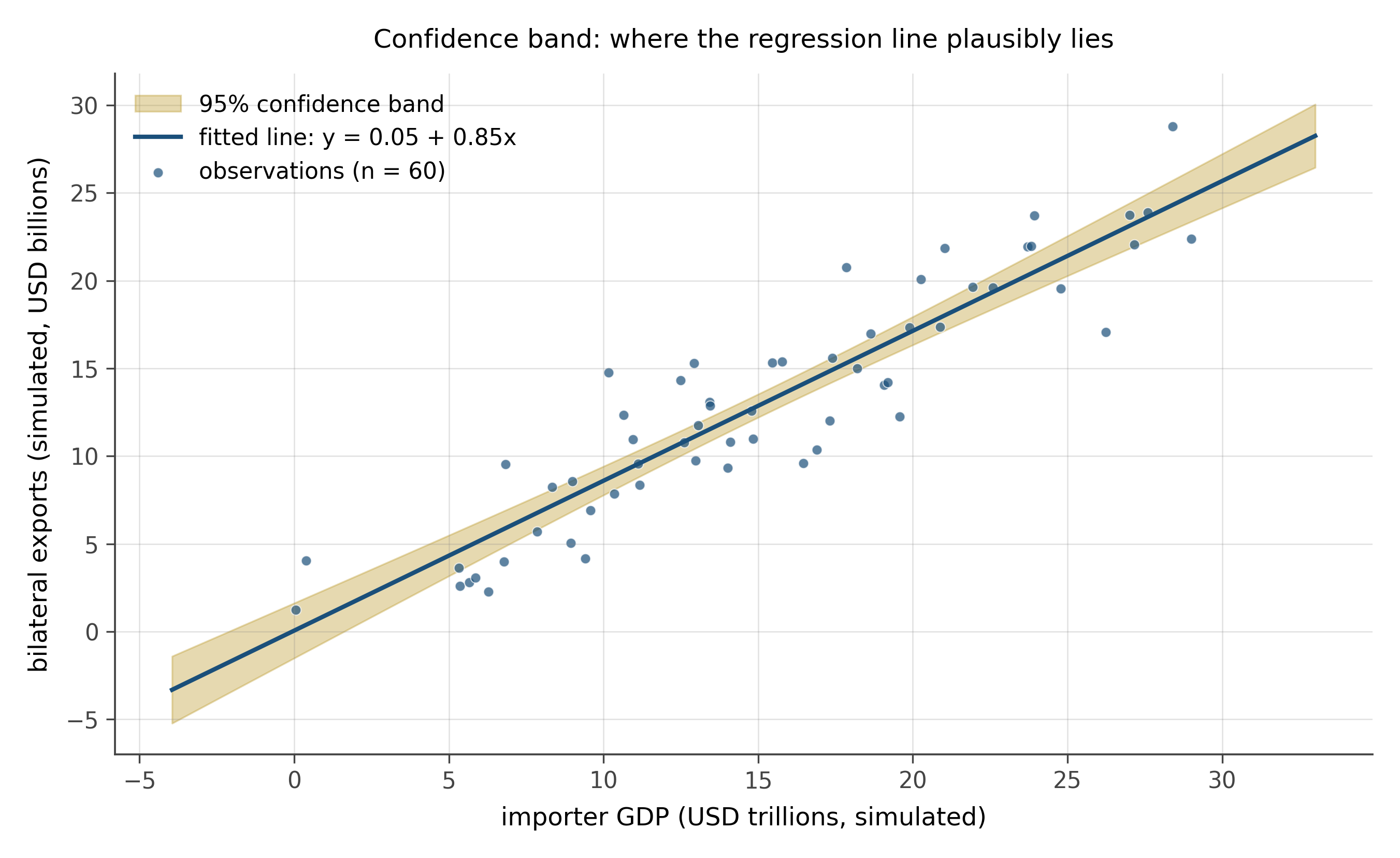
Figure 11.1: A linear regression of bilateral exports on importer GDP, with a 95% confidence band shaded around the fitted line. The band narrows in the dense part of the data and widens at the extremes, which is a faithful encoding of how much the regression line itself is uncertain at each x-value. The wider band beyond the data range is the most honest way to show extrapolation uncertainty.

Two important distinctions:

A confidence band shows the uncertainty around the regression line itself: where the true mean function plausibly lies. A prediction band shows the uncertainty around future observations: where new data points are likely to fall. The prediction band is always wider, because it includes both the uncertainty in the line and the residual scatter around the line. Confusing them is one of the most common errors in applied empirical work.

Confidence bands handle asymmetry naturally. If the true function has heteroskedastic errors, the band can fan out at the edges. They also handle non-linear models easily: a logistic regression’s confidence band on the probability scale is non-symmetric, and the band reflects this. They are the right default for any continuous predictor.

11.3 Coefficient plots

A coefficient plot, also called a forest plot in medicine and meta-analysis, shows many regression estimates at once. Each row is one coefficient. The dot is the point estimate. A horizontal line through the dot is the confidence interval. A vertical reference line, usually at zero, marks the null.

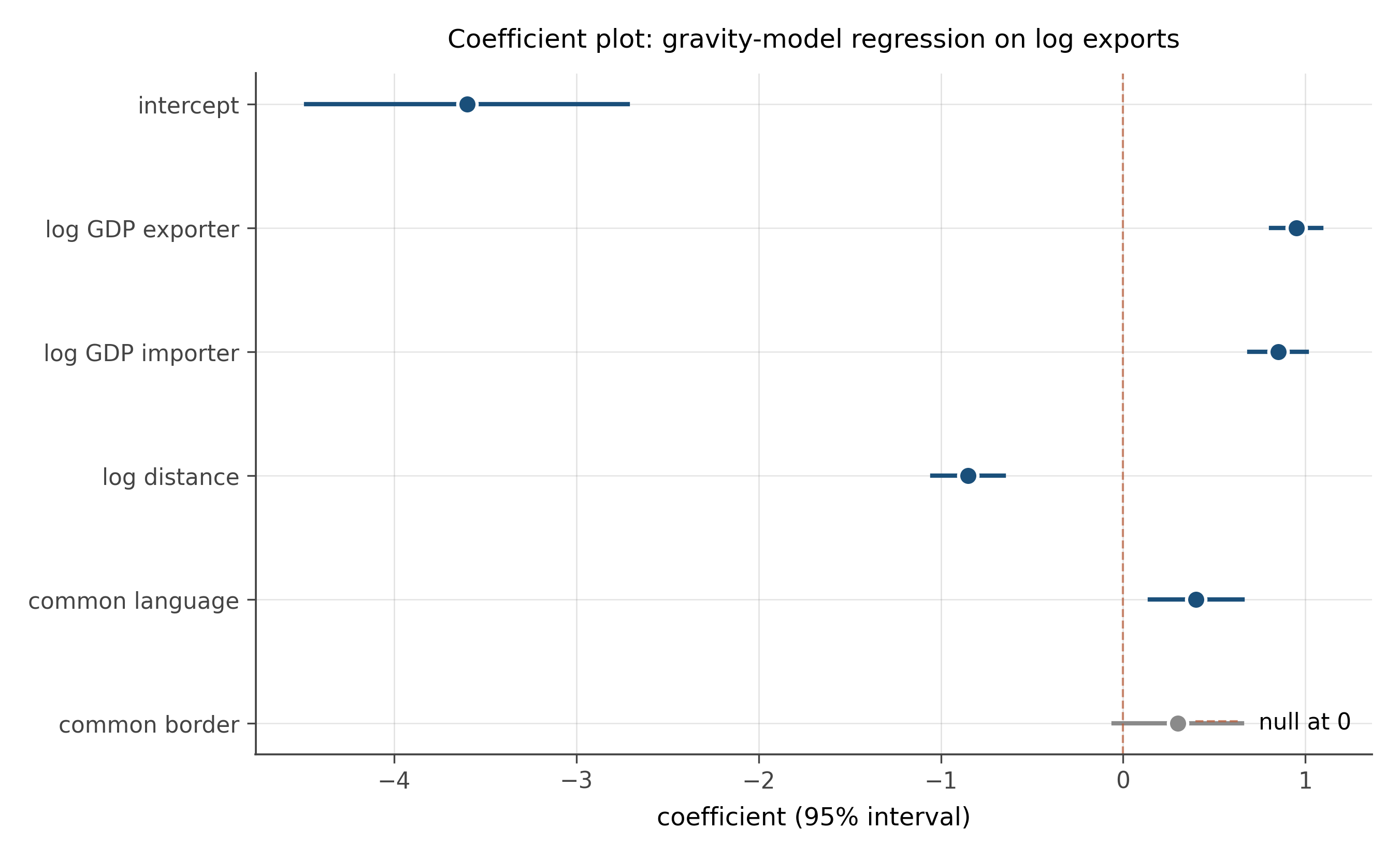
Figure 11.2: Coefficients from a regression of log bilateral exports on log importer GDP, log distance, common-language indicator, and an intercept. Each row is one coefficient with a 95% interval. The vertical line at zero marks the null. Coefficients whose intervals cross the line cannot reject the null at the conventional level; coefficients whose intervals sit clearly to one side are far from zero in their estimated direction.

Why this works better than the standard alternative, a regression table. A regression table displays the same information as numbers in a grid. The numbers require translation: the reader must compare each coefficient to its standard error mentally, decide whether the interval crosses zero, and judge magnitudes by mentally normalizing to the units of each variable. A coefficient plot does all of this visually. The reader sees at a glance which estimates are large, which are precise, which cross zero, and which are similar in magnitude.

Coefficient plots are now standard in modern empirical economics and political science papers, partly because of the credibility revolution and partly because they make it harder to hide weak results in a table of numbers.

11.4 Hypothetical outcome plots

A hypothetical outcome plot, or HOP, shows uncertainty by sampling. Instead of drawing a confidence band, the plot shows several plausible realizations of the underlying quantity, drawn from the posterior or the sampling distribution. In a static figure, an HOP overlays a few dozen sampled curves in light color, with the central estimate in a heavier line. In a dynamic figure (animated, interactive), the HOP cycles through draws over time, giving the reader a visceral sense of how much the estimate could vary.

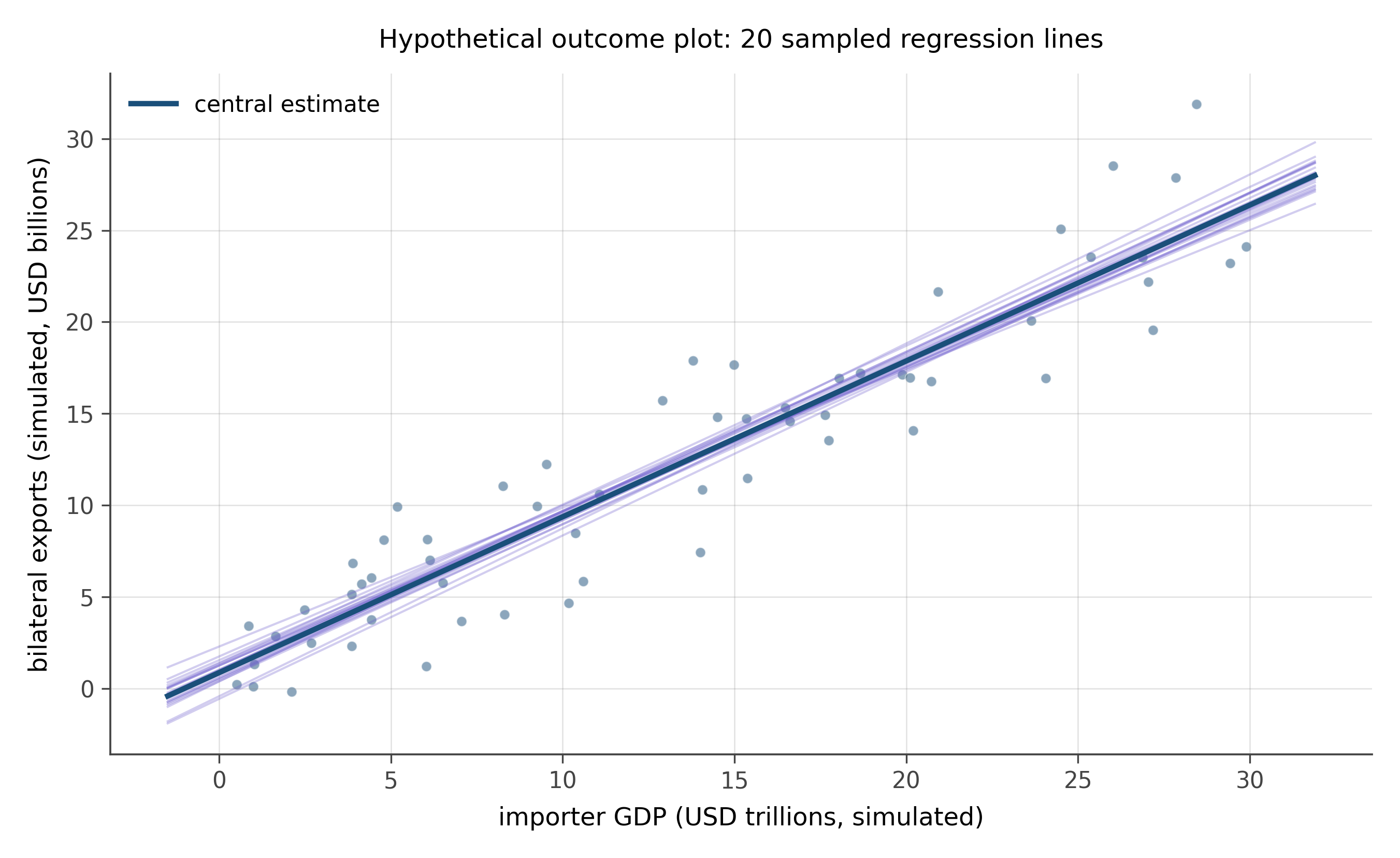
Figure 11.3: Twenty regression lines drawn from the joint distribution of slope and intercept, overlaid on the data. The dark line is the central estimate. Each light line is one plausible realization of the underlying line consistent with the data. The thicker the visible bundle, the less confident the estimate; the spread of the bundle is the uncertainty.

The pedagogical case for HOPs is that confidence bands feel like static facts, whereas HOPs feel like the underlying probabilistic process. Research by Hullman, Kale, and others has shown that HOPs improve viewers’ calibration of subjective beliefs about uncertainty better than equivalent confidence-band displays. The reason is roughly that bands encode a precise probability, but the eye reads “more probable here, less probable here” with mixed accuracy, whereas HOPs encode the same probabilities by the frequency of visual presence, which the eye reads directly.

11.5 Fan charts

A fan chart is a forecast visualization. The forecasted quantity is plotted as a curve into the future, with a series of nested confidence bands around it. The innermost band might be a 50% prediction interval, the next 80%, the outermost 95%. The result looks like a fan opening to the right, narrowest at the present moment and widening into the future.

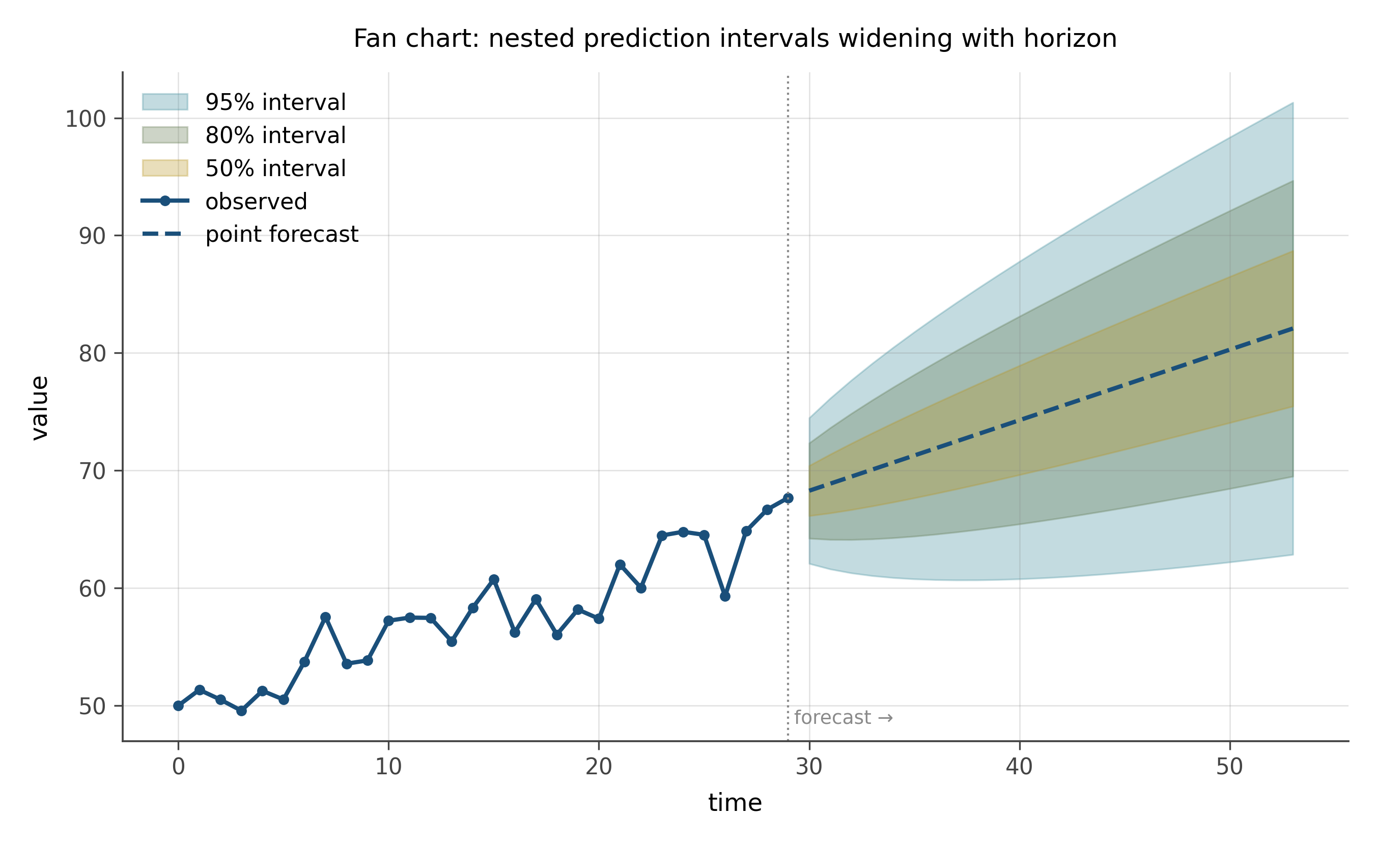
Figure 11.4: A fan chart of a forecasted series. The dark central line is the point forecast; the nested bands are the 50%, 80%, and 95% prediction intervals. The fan widens further into the future, encoding the rate at which forecast uncertainty grows. Bank of England inflation reports use exactly this format; the visual move is to communicate both the central forecast and the rate of uncertainty growth in one figure.

Fan charts are standard in central banking and in epidemiology forecasting. They communicate two things at once: the central forecast (the line in the middle) and the rate at which uncertainty grows (the rate at which the fan opens).

The visual property worth noting: the bands are nested rather than separate. The reader’s eye reads “more probability concentrated in the inner bands, less in the outer ones,” which is the right reading. A single 95% band gives a binary in-or-out reading. A nested fan gives a graded reading: more or less likely.

11.6 Showing all the data

The most honest uncertainty visualization is showing all the data. When sample sizes permit, plot every individual observation as a small mark, with the summary (mean, regression line, model) overlaid. The eye reads both the structure and the spread, and there is no chance of being misled about precision.

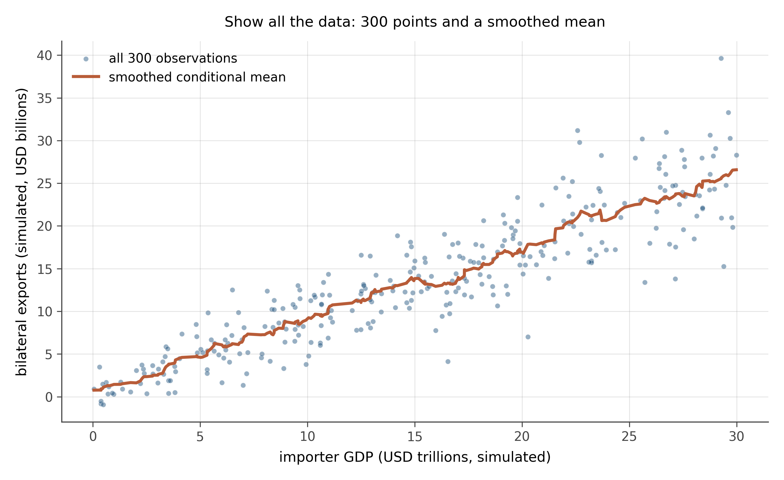
Figure 11.5: Every one of our 300 bilateral observations plotted as a point, with a smoothed conditional mean overlaid. The dispersion of the points around the line is the residual variation. The slope of the line is the estimated relationship. Showing the data and the model together is the most informationally honest visualization of uncertainty available.

This is what scatter plots already do, but the principle generalizes. A box plot shows summary statistics; a strip plot shows summary statistics and every individual observation. A bar chart shows means; a violin or jittered scatter shows means and the underlying spread.

The trade-off. When n is small, “show all the data” is easy. When n is millions, you need to pre-aggregate or use density-based encodings (hex bins, contour plots). The principle stays the same: prefer showing more rather than less, and make explicit the choice about what is hidden.

Key insight

Uncertainty deserves the same care as the point estimate. Error bars are common but rarely optimal: they hide more than they show. Confidence bands, coefficient plots, hypothetical outcome plots, and fan charts each show uncertainty as a first-class part of the visual argument. The general rule: show all the data when you can; where summary is unavoidable, encode the uncertainty in a way that matches the reader’s question.

Try this

A regression of bilateral exports on importer GDP gives a slope estimate of 0.88 with a standard error of 0.06. Sketch:

The result as an error-bar plot.
The result as a coefficient plot, with the null line at 0 and a second null line at 1 (the gravity-model benchmark).
The result as a confidence band over the range of importer GDP in the data.

Compare the three. Which most clearly answers “is the slope different from 1?” Which most clearly answers “how confident am I about the slope at GDP equal to 25 trillion?” Which would you publish?

Inside the math: pointwise vs simultaneous bands

A pointwise 95% confidence band at each x-value gives an interval such that, if you repeated the experiment many times, 95% of the resulting intervals at that x would cover the true mean function. A simultaneous 95% confidence band is wider and gives an interval such that the entire band contains the true function 95% of the time.

These are different things. The pointwise band is the standard default in most software and is what most researchers report. The simultaneous band is what you actually want if you intend to make claims about multiple x-values at once. The simultaneous band can be substantially wider than the pointwise version, especially when the predictor has many evaluation points.

A simple rule of thumb. If you are reporting a single test at a single x, the pointwise band is fine. If you are reporting on an entire curve and might select x-values post hoc, you want the simultaneous band. The Working-Hotelling band is the classical construction; modern bootstrap-based bands are the practical alternative.

Reflect before moving on

Three questions to articulate in your own words:

The chapter claims that error bars on bar charts are usually the wrong choice. In your own words, why? Where have you seen error bars used well?
A confidence band and a prediction band are different. Which one would you want to see if you were asked to forecast where a new observation will land? Which if you were asked about the underlying mean function?
HOPs (hypothetical outcome plots) work because the eye reads frequency directly. Where else in this book have you seen frequency used as a visual encoding?

Frontier note

Modern uncertainty visualization is an active research area. Three directions worth knowing.

Animated and interactive uncertainty. Hypothetical outcome plots, ensemble visualizations, and dynamic confidence regions have been shown by Hullman, Kale, and others to improve viewer calibration of subjective uncertainty. The visualizations on this book’s website use these where they fit.

Multiverse analysis displays. When the same dataset can support many defensible analyses (specification choices, measurement choices, robustness checks), the modern move is to display the distribution of results across all of them. Specification curves and multiverse plots are the two leading visual formats.

Bayesian posterior visualization. Modern Bayesian software produces full posterior distributions. Visualizing those distributions, rather than reducing them to a single CI, is its own active design space. Density plots, eye-plots, and fan-style visualizations are all in current use.

The general direction: less reduction, more information. The trend follows the technical capacity to compute and display the underlying probabilistic objects directly, rather than summarize them away.

11.7 Practice problems

Find a paper in your field that uses error bars on a bar chart. Sketch the same data as a coefficient plot. Which version is more useful for the question the paper is trying to answer?
A 95% confidence band for a regression of y on x is plotted. At x = 5 the band runs from y = 2.4 to y = 3.6. Write one sentence describing what this band means, and one sentence describing what it does not mean.
Take the trade slice. Fit a simple regression of log exports on log importer GDP. Plot it three ways: (a) point estimate plus error bar; (b) confidence band; (c) hypothetical outcome plot with twenty draws. Compare. Which makes the gravity slope feel most uncertain?
A fan chart of disease cases shows the 50%, 80%, and 95% prediction intervals widening into the future. Two months out, the 95% interval spans 100 to 1,000 cases. Is that a useful forecast? When would a fan chart with very wide outer bands still be informative?
Construct a coefficient plot for the multiple-regression result you choose: at minimum three coefficients with their 95% intervals and a vertical reference line at zero. Annotate which coefficients are statistically distinguishable from zero and which are not. The exercise is half the chart and half the writing of the annotations.

Looking ahead

Chapter 9: Reading equations. The previous chapters built up your visual vocabulary. The next chapter builds the matching vocabulary for mathematical notation, which is what carries every formal claim about uncertainty in this book. Continue →