7 The grammar of graphics – Pictures of Inference

7.1 Anatomy of a chart

A chart is not a kind of thing. It is not “a bar chart” or “a scatter plot.” A chart is a recipe with three layers, and once you see the layers separately, the apparent variety of charts collapses into a much smaller set of decisions.

The recipe was named by Leland Wilkinson in 1999 in The Grammar of Graphics, and refined by Hadley Wickham into the ggplot2 implementation in R. Both versions agree on what the layers are.

Data. The dataset you are visualizing. Rectangular, of course. Rows are observations, columns are variables.

Aesthetics. The mapping from columns of the dataset to visual properties of the chart. Position on the x-axis. Position on the y-axis. Color. Size. Shape. Each visual property is called an aesthetic, and the chart-maker decides which dataset variable, if any, gets mapped to each aesthetic.

Geometry. The kind of mark used to render each row. A point. A bar. A line. A polygon.

That is the entire vocabulary. A scatter plot is data + position-x + position-y + point. A bar chart is data + position-x + length-y + bar. A line chart is data + position-x + position-y + line. A faceted small-multiples plot is the same with one extra aesthetic, usually called facet, that splits the data into panels.

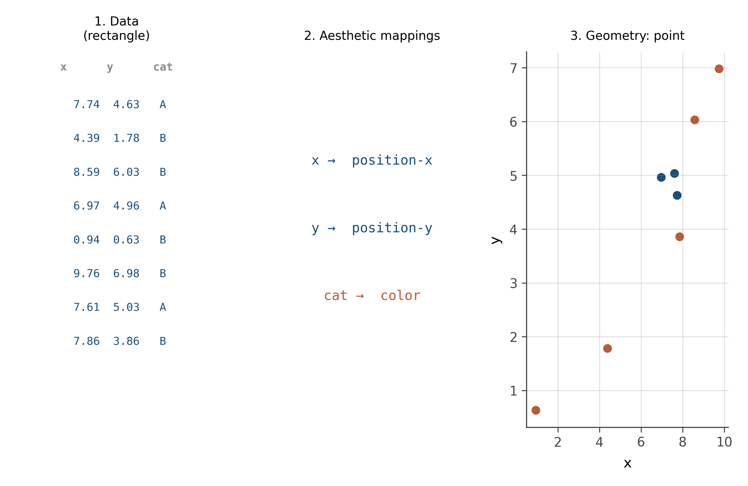
Figure 7.1: Anatomy of a single chart, exploded into the three layers of the grammar. The data is a small slice of trade flows. One row maps to one geometric mark (a point). The aesthetics map columns of the data to visual properties of the mark: x-position, y-position, color. Change the geometry and you get a different chart from the same data and aesthetics.

Once the grammar is in your head, “what kind of chart should I make” stops being a question about chart types and becomes a question about which aesthetic each of your variables should get mapped to. That is the right question. The answer depends on what you want the reader to see, and on what the human visual system is good at.

7.2 The perceptual hierarchy

Not all aesthetics are created equal. The human visual system reads some encodings much more accurately than others, and this fact has been measured carefully.

The hierarchy, from most accurate to least, was established by Cleveland and McGill in 1984 and confirmed in many studies since:

Position along a common axis
Position along non-aligned axes
Length
Angle and slope
Area
Volume
Color hue and density

This means that the same number, encoded as a position on a scatter plot’s y-axis, is read more accurately than the same number encoded as the height of a bar (which is length), much more accurately than the same number encoded as the area of a circle, and far more accurately than the same number encoded as the lightness of a color.

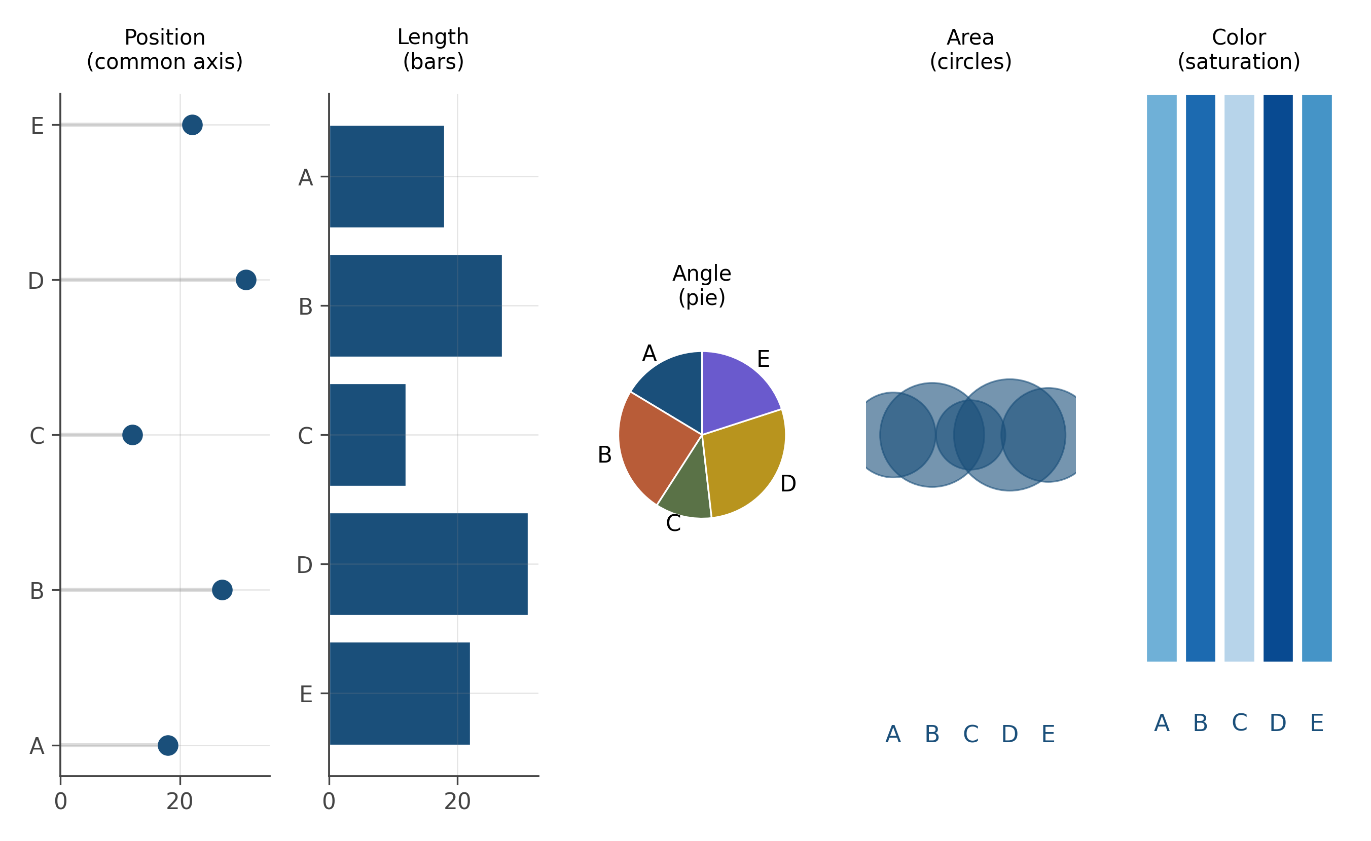
Figure 7.2: The same five values rendered five ways: as positions on a common axis, as bar lengths, as pie-slice angles, as circle areas, and as color values. Cleveland and McGill’s experiments asked subjects to compare encoded values; accuracy fell off in roughly that order. Position is read accurately. Color is read poorly.

The implication is brutal and important. When you have a choice, encode the variable you most want the reader to read accurately as a position. When you do not have a choice (because position is already taken by other variables), use length next. Use area only when ranking the values matters but precise comparison does not. Use color hue last, and only when the variable is categorical or the question is about rough categories.

This is why bar charts are usually fine but pie charts are usually not (the reader compares angles, item 4 on the list, when length on a bar chart, item 3, would be more accurate). It is why bubble charts are misleading (area, item 5). It is why heatmaps work for “spot the hot region” but fail for “compare exact values” (color, the bottom of the list).

7.3 Small multiples

When you have one extra variable beyond what x and y are encoding, you face a choice. Map the extra variable to a within-panel aesthetic (color, shape, size), or use it to split the chart into panels.

Splitting into panels is called faceting, or small multiples, and it has a strong claim to being the most underused visualization technique in working analysis. The design move: instead of overlaying everything on one chart, repeat the chart structure across panels, with each panel showing a slice of the data.

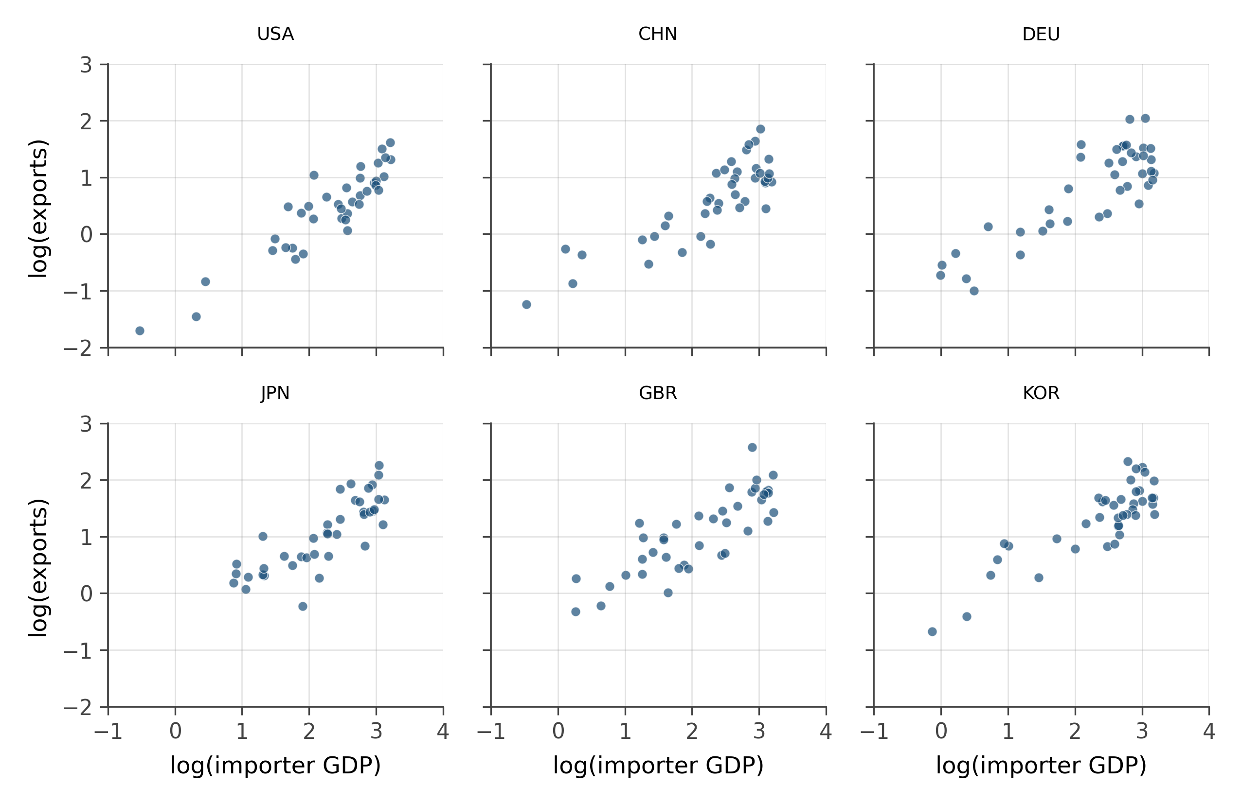
Figure 7.3: A scatter of bilateral exports against importer GDP, faceted by exporter country. Each panel uses the same axes and the same encoding; only the panel-defining variable changes. The pattern in any one panel is easy to read, and so is the contrast across panels. The same data overlaid in one panel with color-by-country would be a tangled mess.

Small multiples work because they use position (the panel grid is a position encoding) for the splitting variable, and they keep the within-panel encoding clean. They also support the eye in moving across panels: if all panels share axes, the visual comparison is doing the same kind of work as a scatter plot of summary statistics, except every individual data point is visible.

When in doubt, facet.

7.4 The POI palette as semantic vocabulary

This book uses a fixed set of seven colors, and each one carries meaning. The meanings are taught here and respected for the rest of the book.

Color	Hex	Meaning
INK	`#1a4f7a`	primary, default, the main story
RUST	`#b85c38`	treatment, contrast, the alternative perspective
SAGE	`#5a7247`	control, comparison, the baseline
GOLD	`#b8941e`	highlighted, derived, the synthesized quantity
VIOLET	`#6a5acd`	uncertain, predicted, the model’s guess
DIM	`#8a8a8a`	background, de-emphasized, support
TEAL	`#3a8a99`	alternative or secondary contrast

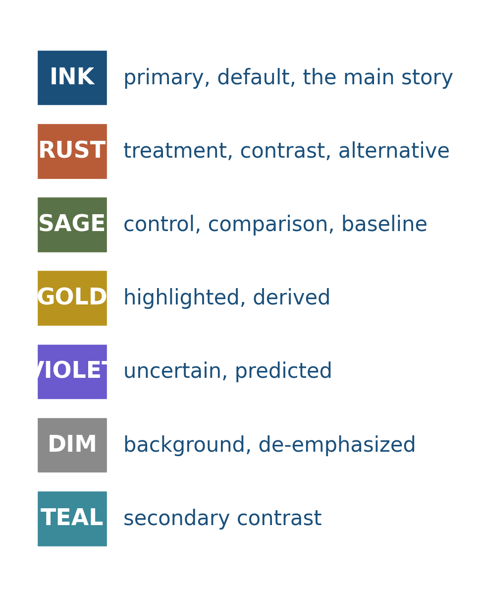
Figure 7.4: The book’s palette as swatches with semantic labels. By chapter five you will recognize the colors without thinking. A new figure with INK and RUST tells you, before you read the caption, that there is a primary story and a contrast. A figure where INK fades to DIM tells you which thing is being de-emphasized.

This is unusual in textbooks. Most books pick colors per chapter, often from a default palette that has no meaning attached. The result is that the reader processes color afresh on every figure, which slows reading and dilutes argument. The palette here is doing real work, and so are you when you respect its conventions while making your own figures.

7.5 Same data, four ways

Here is one small dataset rendered as four different geometries. The data is identical. The aesthetic mappings (which column maps to x and which to y) are identical. Only the geometry changes.

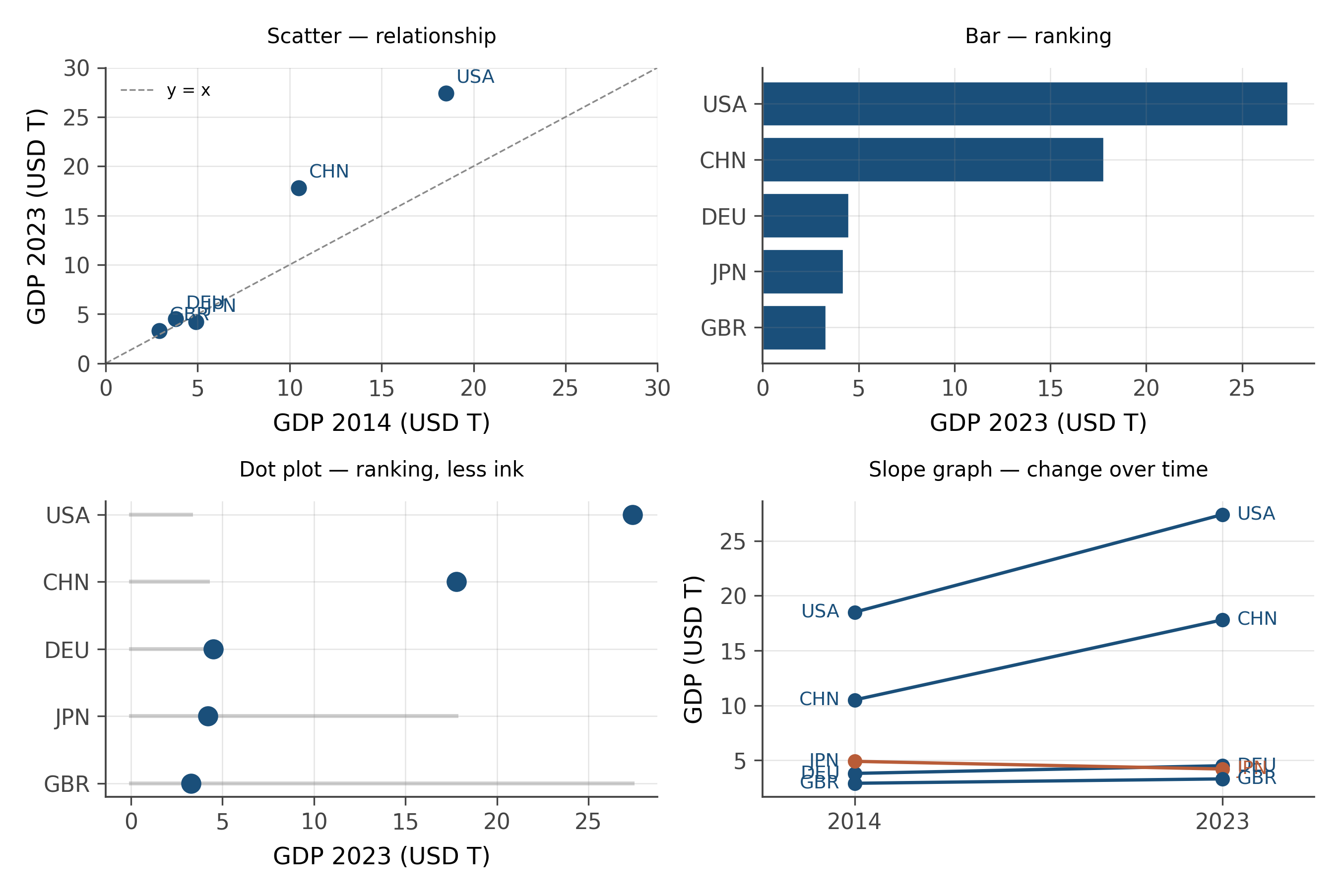
Figure 7.5: One small dataset rendered four ways: scatter, bar, dot plot, slope graph. Each one is correct. Each one privileges a different question. The scatter is good for “how do x and y relate.” The bar chart is good for “rank these from largest to smallest.” The dot plot is the same comparison without the visual weight of bars. The slope graph is good for “how did things change between two points in time.”

Each one is correct. Each one is also, in a sense, wrong, because each one privileges a particular kind of question. The lesson is not that one of these is the best. The lesson is that the choice of geometry is a substantive choice about which question the chart is designed to answer.

When you make a chart, ask first: what does the reader need to see? That answer chooses the geometry. Everything else follows.

Key insight

A chart is data plus aesthetic mappings plus geometry, in that order. Changing the geometry without changing the data answers a different question. Changing the aesthetic mappings without changing the geometry is what most “chart improvement” actually consists of. The perceptual hierarchy (position beats length beats angle beats area beats color) is the constraint that decides which mappings serve the reader and which do not.

Try this

Pick any chart from a recent news article. Identify the three layers: what is the dataset, which columns are mapped to which aesthetics, and what is the geometry?

Then ask: would another geometry, with the same data and aesthetics, answer the question better? Would a different aesthetic mapping (color instead of x-position, say) work better, given what the reader is supposed to see?

The exercise gets faster with practice. By the tenth chart you will be doing it automatically.

Inside the math: a more formal grammar

Wilkinson’s Grammar of Graphics (1999) decomposed a chart into seven layers, of which the three above are the most consequential. The full list adds scales (how data values are mapped to visual values), coordinates (Cartesian, polar, geographic projections), facets (the small-multiples splitting variable), and themes (typography, gridlines, palette). Wickham’s ggplot2 implementation in R follows the same structure.

The grammar is more general than this chapter’s three-layer simplification suggests. A polar coordinate system applied to a bar chart produces a pie chart (with all the perceptual liabilities described above). A logarithmic scale applied to a continuous axis produces a log-log plot. A geographic projection applied to a position aesthetic produces a map.

Each move is a transformation in the grammar, and the same chart is described compactly by the sequence of transformations rather than by a chart-type name. This is the conceptual move that makes ggplot2 readable to people who have never seen it: the syntax mirrors the grammar.

Frontier note

The grammar of graphics is now several decades old and the field has moved on. Three directions worth knowing.

Interactive grammars. Vega and Vega-Lite extend the static grammar to interaction (brushing, linked views, animation). The visualizations on this book’s website use Observable Plot, which is in the same family. The interactive grammar is largely the static grammar plus a vocabulary for events and selections.

Algebraic visualization grammars. Recent work by Wills, Pu, and others has formalized the grammar as an algebra, where chart compositions can be reasoned about systematically. This is the basis for tools that auto-recommend visualizations given the data.

Perceptual grammars. Modern work continues to refine Cleveland and McGill’s hierarchy with new experimental data, especially for unconventional encodings (animated transitions, 3D, AR/VR). Most of the new findings reinforce the original hierarchy with caveats. Position remains king.

The grammar is not finished, but the foundation is stable enough that this book will rest on it without apology.

7.6 Practice problems

Take any chart from a recent news article. Identify the data, the aesthetic mappings, and the geometry.
You have country, year, GDP, and continent. Sketch a chart that uses all four variables. Justify each encoding choice using the perceptual hierarchy.
Why is a pie chart usually a worse choice than a bar chart for the same comparison, even when both encode the same data?
Faceting moves an aesthetic from within-panel to position-of-panel. Explain why that is often an improvement, in terms of the perceptual hierarchy.
Take the trade slice. Make four versions of the same scatter (exports vs distance), encoding exporter four different ways: as color, as shape, as size, as facet. Which encoding lets you read the data fastest?

Reflect before moving on

What is one chart you have made or seen recently that violates the perceptual hierarchy? Could it be redrawn?
Color is at the bottom of the hierarchy but is used everywhere. Why? When is color actually justified?
Pick a question you have had to answer with data and name the right geometry for it.

Looking ahead

Chapter 5: Center, spread, shape. The grammar tells you how to encode. The next chapter turns to the question of what to encode: the descriptive statistics that survive contact with reality. Mean and median, variance and IQR, robustness as a working concept. Continue →