5 Probability as area – Pictures of Inference

5.1 What probability is

Pause on the word “probability.” Pretend you have never heard it before. What kind of thing is it?

Here is the answer the book will use, and it is the answer modern probability theory uses too: probability is a fraction of an outcome space.

That sentence does a lot of work. Let me unpack it slowly.

An outcome space is the set of all the things that could happen in some situation. When you roll a fair die, the outcome space is the six numbers from 1 to 6. When you draw a card from a shuffled deck, the outcome space is the 52 distinct cards. When you flip a coin, the outcome space has two elements. When you measure tomorrow’s high temperature in Atlanta, the outcome space is technically every real number between some lower and upper bound, an infinite continuum.

Once you have an outcome space, probability is just bookkeeping over the space. The probability of any specific outcome is a number between 0 and 1. Add up the probabilities of the outcomes inside any subset, and you get that subset’s probability. The probability of the whole space is exactly 1, because something has to happen.

That is it. There is a deeper formal version with σ-algebras and measure theory waiting later in the book, but at this level, probability is “what fraction of the things that could happen does this subset cover.”

The picture below, and the rest of this chapter, takes that definition seriously.

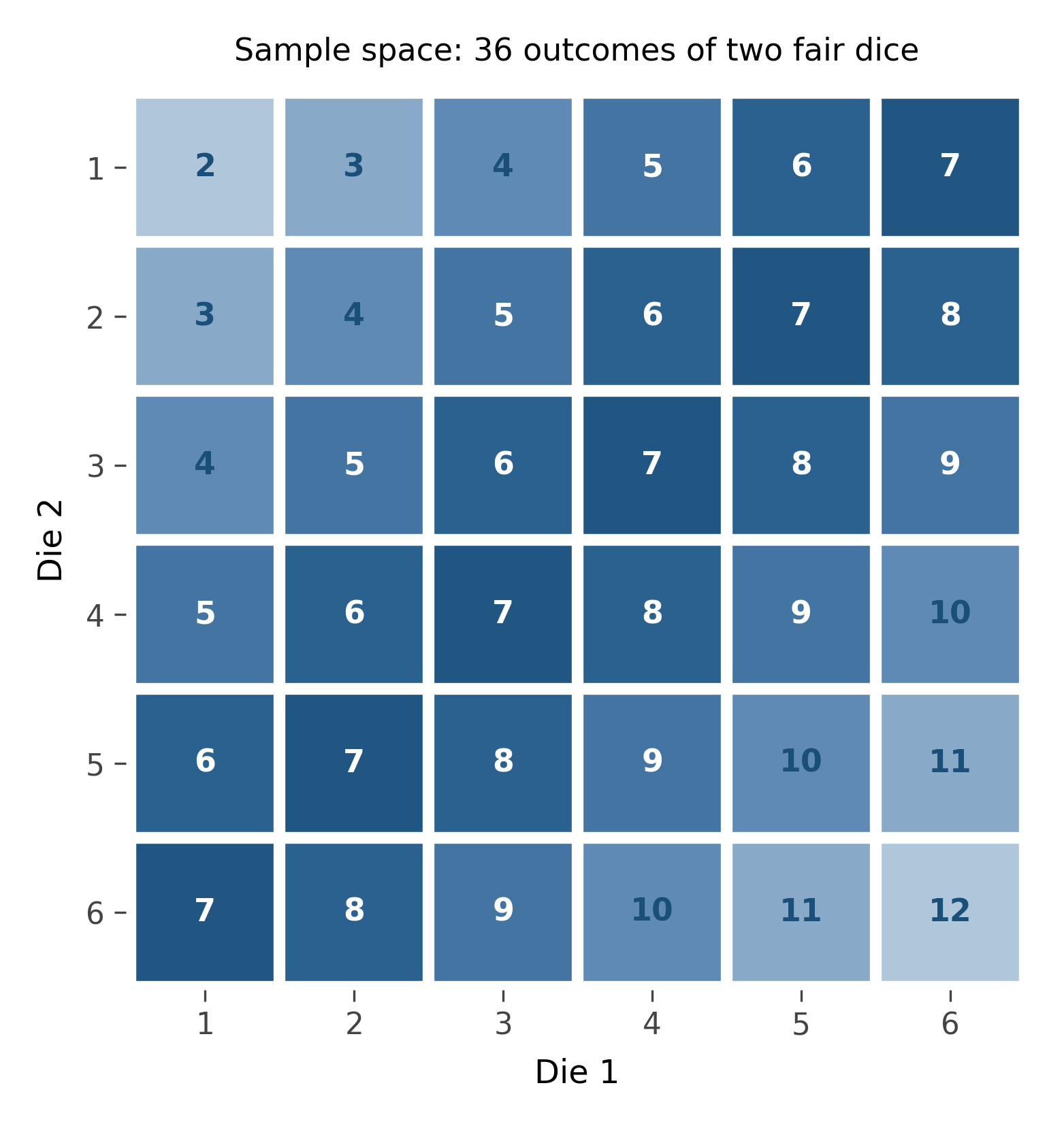
Figure 5.1: Every outcome of rolling two fair dice. There are 36 cells, one for each ordered pair of die-1 and die-2 values, and the number in each cell is the sum. The shading shows how many cells share the same sum: the diagonal stripe with sum 7 has six cells, sum 6 and sum 8 have five, and so on, down to sums 2 and 12 with one cell each. Probability becomes geometry: the chance of rolling a 7 is just the fraction of the rectangle that is shaded most darkly.

Notice what the picture does not yet have: any equation. Probability is not, fundamentally, an equation. It is a way of carving up a space. The equations come later, as shorthand for the carving.

The same idea works whether the space is finite or continuous. When you throw a dart at a square dartboard, the outcome space is the dartboard itself. The probability that the dart lands in some region is the fraction of the dartboard that region covers. This is literally area divided by area, no abstraction required.

When you measure tomorrow’s temperature, the outcome space is a number line and the probabilities are encoded by a density: a curve over the number line whose total area equals 1. The probability that the temperature lands in some interval is the area under the density curve over that interval. We will spend chapter three meeting the most important density curves and learning to read them. For now, the only thing to remember is that area under a curve is probability. Always. No exceptions.

5.2 Events are regions

An event is just a name for a subset of the outcome space.

“The card I draw is a heart” is an event. It corresponds to the subset of the deck consisting of the 13 hearts. The probability of the event is 13/52, or 1/4, because the heart-region covers a quarter of the deck.

“The card is a face card” (jack, queen, king of any suit) is another event. It corresponds to 12 cards out of 52. Probability 12/52, about 0.23.

What about “the card is a heart and a face card”? That is the intersection of the two events: the cards that are simultaneously hearts and face cards. There are exactly three of those (jack, queen, king of hearts). Probability 3/52, about 0.058.

What about “the card is a heart or a face card”? That is the union. You might be tempted to add the two probabilities, 13/52 + 12/52 = 25/52. That is wrong, and the reason it is wrong is one of the most useful diagrams in elementary probability.

The hearts and the face cards overlap. The three cards in the intersection (J, Q, K of hearts) belong to both regions. If you add 13 and 12, you have counted those three twice. To get the union, you add the two regions and subtract the overlap once:

P(\text{heart} \cup \text{face}) = P(\text{heart}) + P(\text{face}) - P(\text{heart} \cap \text{face}) = \frac{13}{52} + \frac{12}{52} - \frac{3}{52} = \frac{22}{52}.

This is the inclusion-exclusion principle, and it has a name only because beginners get it wrong so often. The picture is unambiguous.

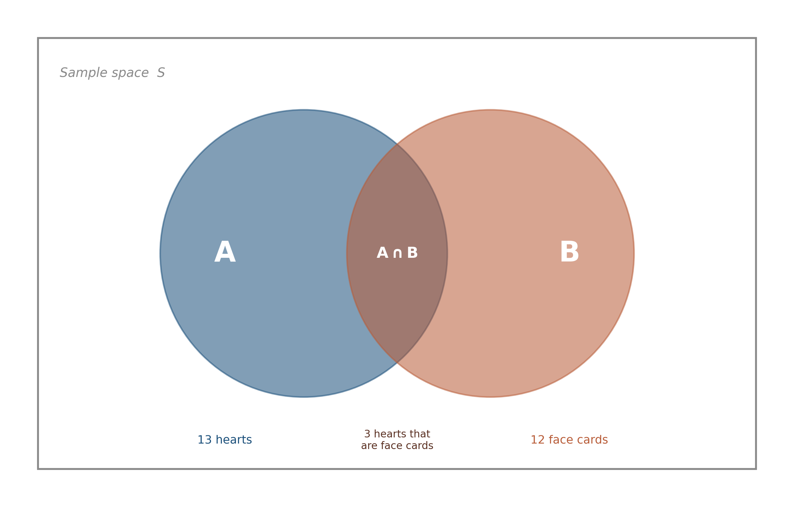
Figure 5.2: Two events drawn as overlapping regions inside a rectangular sample space. The blue region A is “the card is a heart” (13 of 52). The rust region B is “the card is a face card” (12 of 52). The overlap A ∩ B has three cards (J, Q, K of hearts). When you compute P(A ∪ B), the overlap is counted once in P(A) and once in P(B), which means you must subtract it once to avoid double-counting.

Two events that don’t overlap are called disjoint, or mutually exclusive. For disjoint events, the union really is just the sum, because there is nothing to subtract. Drawing a heart and drawing a club are disjoint: no card is both. P(heart or club) = 13/52 + 13/52 = 26/52, exactly half the deck.

Read the figure carefully. Every claim in the next two chapters can be derived from looking at it.

5.3 Conditional probability is a change of denominator

Suppose you draw a card and someone tells you, before you look, that the card is a heart. Now what is the probability the card is a face card?

The original outcome space was 52 cards, of which 12 were face cards. P(face) = 12/52, about 0.23. But you have new information: the card is a heart. The outcome space has shrunk. Instead of 52 cards, only the 13 hearts are now possibilities. Among those 13, exactly 3 are face cards (J, Q, K of hearts). The probability that the card is a face card given that it is a heart is 3/13, about 0.23.

Conditioning on a piece of information is just zooming in. You take the original outcome space, restrict it to the region you have been told about, and recompute the fraction.

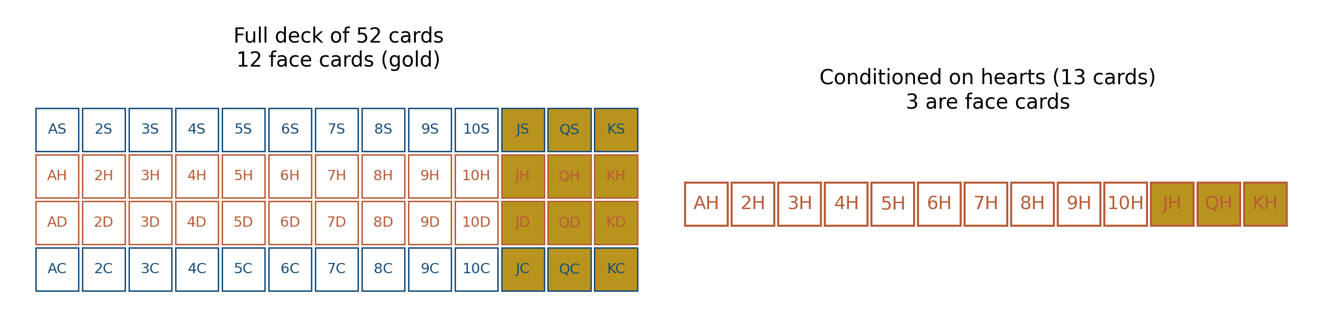
Figure 5.3: Left: the full deck, with the 12 face cards highlighted in gold. The probability of a face card, P(face), is 12/52 ≈ 0.23. Right: the same problem, restricted to the 13 hearts only. The probability of a face card given that the card is a heart, P(face given heart), is 3/13 ≈ 0.23. Conditioning on “heart” zoomed the sample space from 52 cards to 13. The numerator and denominator both changed; in this case the ratio happens to come out about the same.

Notation. The probability of A given B is written P(A \mid B), read aloud as “the probability of A given B.” The vertical bar means “given.” It is the most important piece of notation in inferential statistics, and most students never learn to read it aloud confidently. Read it aloud now.

The formula corresponding to the picture is

P(A \mid B) = \frac{P(A \cap B)}{P(B)}.

Read the formula aloud. The probability of A given B equals the probability of A and B together, divided by the probability of B. In words: of all the times B happened, what fraction of them also had A happen?

Verify it on the cards. P(\text{face} \mid \text{heart}) = P(\text{face} \cap \text{heart}) / P(\text{heart}) = (3/52) / (13/52) = 3/13. Same answer the picture gave. The formula and the picture are saying the same thing in different languages.

Internalize this: P(A \mid B) is a different quantity from P(A). The two probabilities can be very different. Sometimes B raises the chance of A; sometimes B lowers it. When the two probabilities happen to be equal, A and B are independent, and B carries no information about A. The same word “probability” is doing very different work in P(A) and P(A \mid B), and a great deal of statistical confusion in the wild comes from people sliding between them without noticing.

5.4 Bayes and the disease-test paradox

Here is a question that broke me the first time I saw it, and that I have watched humble dozens of trained scientists since.

A rare disease affects 1% of the population. A test for the disease is 95% accurate: among people who have the disease, the test correctly flags 95% of them; among people who do not have the disease, the test correctly clears 95% of them. You take the test. It comes back positive.

What is the probability you have the disease?

Most people, when surveyed, answer somewhere between 90% and 95%, anchoring on the test’s accuracy. The actual answer, as the picture below makes obvious, is roughly 16%.

Casscells, Schoenberger, and Graboys (1978) ran exactly this question on a sample of physicians and house officers at Harvard Medical School. The median answer was 95%. Eddy (1982) later documented similar errors among practicing physicians making real diagnostic decisions. Base-rate neglect is not a layperson’s mistake; it is a working clinician’s mistake too.

Imagine 10,000 people drawn at random from the population. The picture shows them as a 100-by-100 grid of squares.

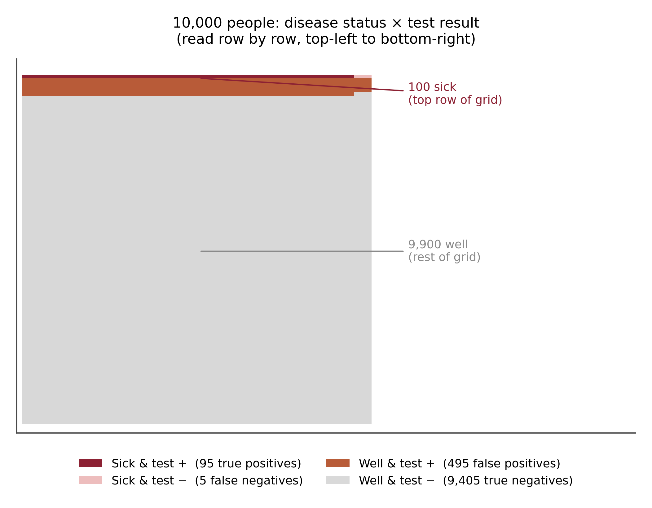
Figure 5.4: 10,000 people, drawn at random from a population with 1% disease prevalence and tested with a 95%-accurate test. The dark red squares are sick people who tested positive (95). The pale red squares are sick people who tested negative (5). The rust squares are healthy people who tested positive anyway, the false positives (495). The gray squares are healthy people who tested negative (9,405). The probability of being sick given a positive test is the fraction of the positive-test population that is also in the sick population: 95 out of (95 + 495) = 590, or about 16%. The base rate dominates.

Of the 10,000 people, 1% have the disease. That is 100 people. The other 9,900 do not.

Among the 100 sick people, the test correctly identifies 95% as positive. That is 95 true positives. The other 5 are false negatives.

Among the 9,900 well people, the test correctly clears 95%. That is 9,405 true negatives. But it incorrectly flags 5%. That is 495 false positives.

Now your test is positive. You belong to the population that tests positive. That population has two parts: the 95 true positives (sick) and the 495 false positives (well). The whole positive-test population is 590 people.

Of those 590, only 95 are actually sick. The probability that a positive-test person has the disease is 95/590, about 0.161, about 16%.

The 95% accuracy did not lie. It just answered a different question. P(+ \mid \text{sick}) = 0.95 is not the same number as P(\text{sick} \mid +). The base rate, that 99% of the population is well, dominates the calculation. With a rare disease and a test that is anything less than perfect, most positives are false positives.

This is Bayes’ theorem, and the formula version is

P(\text{sick} \mid +) = \frac{P(+ \mid \text{sick}) \, P(\text{sick})}{P(+)} = \frac{0.95 \times 0.01}{0.95 \times 0.01 + 0.05 \times 0.99} \approx 0.161.

Read it aloud. The probability of being sick given a positive test equals the probability of testing positive given sickness, times the prevalence of sickness, divided by the total probability of testing positive. That denominator is just the size of the positive-test population (the 590 from the picture), expressed as a fraction.

The formula and the picture say exactly the same thing. The picture is more honest. When you read about Bayes’ theorem in any later chapter, picture the grid first and translate the formula into rectangles second. That is the pedagogical move that prevents an entire class of mistakes that even careful researchers continue to make.

5.5 Move the dials yourself

The grid above used 1% prevalence and 95% test accuracy. The widget below lets you set those parameters yourself. Drag the sliders, watch the colored regions resize, and see how the positive predictive value, P(\text{sick} \mid +), changes.

viewof prevalence = Inputs.range([0.001, 0.50], { value: 0.01, step: 0.001, label: "Disease prevalence" })
viewof sensitivity = Inputs.range([0.50, 0.999], { value: 0.95, step: 0.005, label: "Test sensitivity" })
viewof specificity = Inputs.range([0.50, 0.999], { value: 0.95, step: 0.005, label: "Test specificity" })

ppv = (sensitivity * prevalence) /
      (sensitivity * prevalence + (1 - specificity) * (1 - prevalence))

n_total = 10000
n_sick = Math.round(prevalence * n_total)
n_sick_pos = Math.round(sensitivity * n_sick)
n_sick_neg = n_sick - n_sick_pos
n_well = n_total - n_sick
n_well_pos = Math.round((1 - specificity) * n_well)
n_well_neg = n_well - n_well_pos
n_pos = n_sick_pos + n_well_pos

result_html = html`<div class="poi-bayes-result">
P(sick | positive) = <strong>${(ppv * 100).toFixed(1)}%</strong><br>
<span class="poi-bayes-detail">${n_sick_pos.toLocaleString()} true positives out of ${n_pos.toLocaleString()} positive tests, in 10,000 people.</span>
</div>`

squares = {
  const arr = []
  for (let i = 0; i < n_total; i++) {
    let cls
    if (i < n_sick_pos) cls = "Sick · test +"
    else if (i < n_sick) cls = "Sick · test −"
    else if (i < n_sick + n_well_pos) cls = "Well · test +"
    else cls = "Well · test −"
    arr.push({ x: i % 100, y: Math.floor(i / 100), cls })
  }
  return arr
}

bayes_chart = Plot.plot({
  width: 600,
  aspectRatio: 1,
  marginTop: 36, marginBottom: 8, marginLeft: 4, marginRight: 4,
  x: { axis: null, domain: [-0.5, 99.5] },
  y: { axis: null, domain: [-0.5, 99.5], reverse: true },
  color: {
    domain: ["Sick · test +", "Sick · test −", "Well · test +", "Well · test −"],
    range: ["#8c2329", "#e8bdbd", "#b85c38", "#d8d3c5"],
    legend: true
  },
  marks: [
    Plot.dot(squares, { x: "x", y: "y", fill: "cls", r: 2.7, stroke: null })
  ]
})

Try the rare-disease scenario from the chapter (prevalence 0.01, sensitivity 0.95, specificity 0.95): the PPV is about 16%. Now slide prevalence to 0.10, a much more common condition. The PPV jumps to about 68%. Same test, different world. The base rate dominates the calculation, and the widget makes that fact tangible in a way the static figure cannot.

Key insight

Probability is a fraction of an outcome space. Conditioning is restricting that space. Bayes’ theorem is the bookkeeping that connects the two, and the rectangle-grid picture in this chapter is the only intuition you need to apply it correctly in the simple case.

Try this

A different version of the disease test problem. The disease prevalence is 50% (very common). The test accuracy is the same 95%.

Without computing anything, predict whether P(\text{sick} \mid +) is closer to 50% or 95%.

Then draw the grid. Then compute the answer. Compare to your prediction. Notice how much the prevalence is doing in this problem, even though the prevalence never appears in the test’s specifications.

A second one. Same 1% prevalence as before, but now imagine the test is 99% accurate (99% sensitivity, 99% specificity). Recompute P(\text{sick} \mid +). What changed and what didn’t?

Inside the math: Bayes from first principles

The chapter derived Bayes’ theorem from a picture. Here is the same derivation in symbols, for readers who want to see why it always works.

The conditional probability formula P(A \mid B) = P(A \cap B) / P(B) can be rearranged into P(A \cap B) = P(A \mid B) \, P(B). This is sometimes called the multiplication rule. Notice that the same intersection A \cap B can be written by conditioning the other direction: P(A \cap B) = P(B \mid A) \, P(A). Setting the two equal,

P(A \mid B) \, P(B) = P(B \mid A) \, P(A),

and dividing both sides by P(B) gives Bayes’ theorem in its simplest form,

P(A \mid B) = \frac{P(B \mid A) \, P(A)}{P(B)}.

The denominator P(B) is the marginal probability of B, and in problems like the disease test it is computed by summing over the conditioning variable: P(B) = P(B \mid A) P(A) + P(B \mid \text{not } A) P(\text{not } A). This is the law of total probability, and it is the formal version of “add up the squares in the grid that meet condition B.”

That is the entire mathematical content of Bayesian inference. Everything that follows in chapters 30 and beyond is just turning the rectangles into curves and the counts into integrals.

Frontier note

Modern Bayesian statistics is the largest practical descendant of the simple bookkeeping you just learned. A working Bayesian analysis turns the rectangle picture from this chapter into a continuous version (the rectangles become curves and the counts become integrals), and asks the same question: given the data, what is the conditional distribution of the parameters?

The recent renaissance of Bayesian methods in applied work owes most of its momentum to two things: better computational tools (Hamiltonian Monte Carlo, variational inference), and a slow shift in scientific culture toward thinking about uncertainty in the way Bayes’ theorem requires.

For now, every time you condition on data in this book, remember that you are doing a tiny piece of Bayesian thinking, even if the chapter calls it something else.

5.6 Practice problems

A bag has 5 red, 3 blue, and 2 green marbles. You draw one. Compute P(\text{red}), P(\text{blue or green}), and P(\text{red and blue}). Sketch the sample space as a rectangle to verify.
Repeat the disease-test problem with prevalence 5% and test accuracy 90% (90% sensitivity, 90% specificity). Draw the grid for 10,000 people and compute P(\text{sick} \mid +).
Two events A and B have P(A) = 0.4, P(B) = 0.5, P(A \cap B) = 0.1. Compute P(A \cup B), P(A \mid B), and P(B \mid A). Are A and B independent?
Why is P(A \cup B) = P(A) + P(B) - P(A \cap B) rather than just P(A) + P(B)? Explain in one sentence and a small picture.
A test has 99% sensitivity and 99% specificity, and the underlying disease has prevalence 0.1%. Without computing, predict whether P(\text{sick} \mid +) is closer to 99% or 10%. Then compute and compare.

Reflect before moving on

What is the visual difference between conditional probability and joint probability?
Where else in the world have you seen base-rate neglect at work?
If a friend asked you “what is probability, in one sentence,” what would you say now that you could not have said before this chapter?

Looking ahead

Chapter 3: Shapes of data. Probability lets you assign a number between 0 and 1 to a region of an outcome space. The next chapter asks: what shapes do real data actually take? Six distributions, each one a story about the kind of process that produces it, each one a tool you will reach for repeatedly for the rest of the book. Continue →