6 Shapes of data
- Six distributions as stories about the processes that produce them
- The 68-95-99.7 rule for the normal
- Why heavy tails matter and how to recognize them
- When to log-transform right-skewed data
6.1 What a distribution is
You have a column. A few hundred rows of bilateral exports, or trade distances, or human heights, or wait times for the bus. The values are not all the same, and they are not arranged at random across some flat range. They cluster, they spread, they trail off. The pattern of where the values fall is what statisticians call the distribution.
A distribution is the answer to “for any given value, how often does it appear?” If you collect heights of adult men in centimeters and bin them into one-centimeter buckets, you can plot the count in each bucket and watch a shape emerge. The shape is not random. It has a name. It carries information about the kind of process that produced the values.
Most of the conceptual work of statistics is recognizing distribution shapes and matching them to processes. You learn the half-dozen most important shapes and which kinds of real-world situations produce them, and a great deal of the rest of the field becomes the question of how to use those shapes to make good decisions.
This chapter introduces six distributions you will see repeatedly. None of them are formulas to memorize. Each is a story: a description of what generates data with this shape. When you meet a column of numbers in the wild, your first move is to ask what story produced it. The right answer points at the right tool.
Six stories follow. Each gets a figure. Read the figures first, the prose second.
6.2 Bernoulli and binomial: a coin and a tally
Start with the simplest possible distribution. You have a single yes-or-no event with probability p of being yes. Coin flip with a biased coin. Click-or-no-click on an ad. Whether a randomly chosen person owns a passport. The outcome is one of two values, conventionally encoded as 1 (yes) and 0 (no). The distribution is called Bernoulli, and it is fully described by the single number p.
You can plot a Bernoulli distribution as two bars: one of height p at the value 1, one of height 1-p at the value 0. That is the entire shape. There is nothing more to know.
Now suppose you do n independent Bernoulli trials with the same p and count how many came out yes. The number of yeses is no longer a yes-or-no; it is an integer between 0 and n. The distribution of that count is called binomial, written Binomial(n, p). It has more shape than the Bernoulli does, because the count can land anywhere in a range, and some counts are far more likely than others.
When n is small, the binomial is asymmetric and lumpy. When n is large, it starts to look like a bell curve centered at np with width controlled by \sqrt{np(1-p)}. We will return to that “starts to look like” later in the book, because it is one of the most important facts in statistics. For now, recognize the shape.
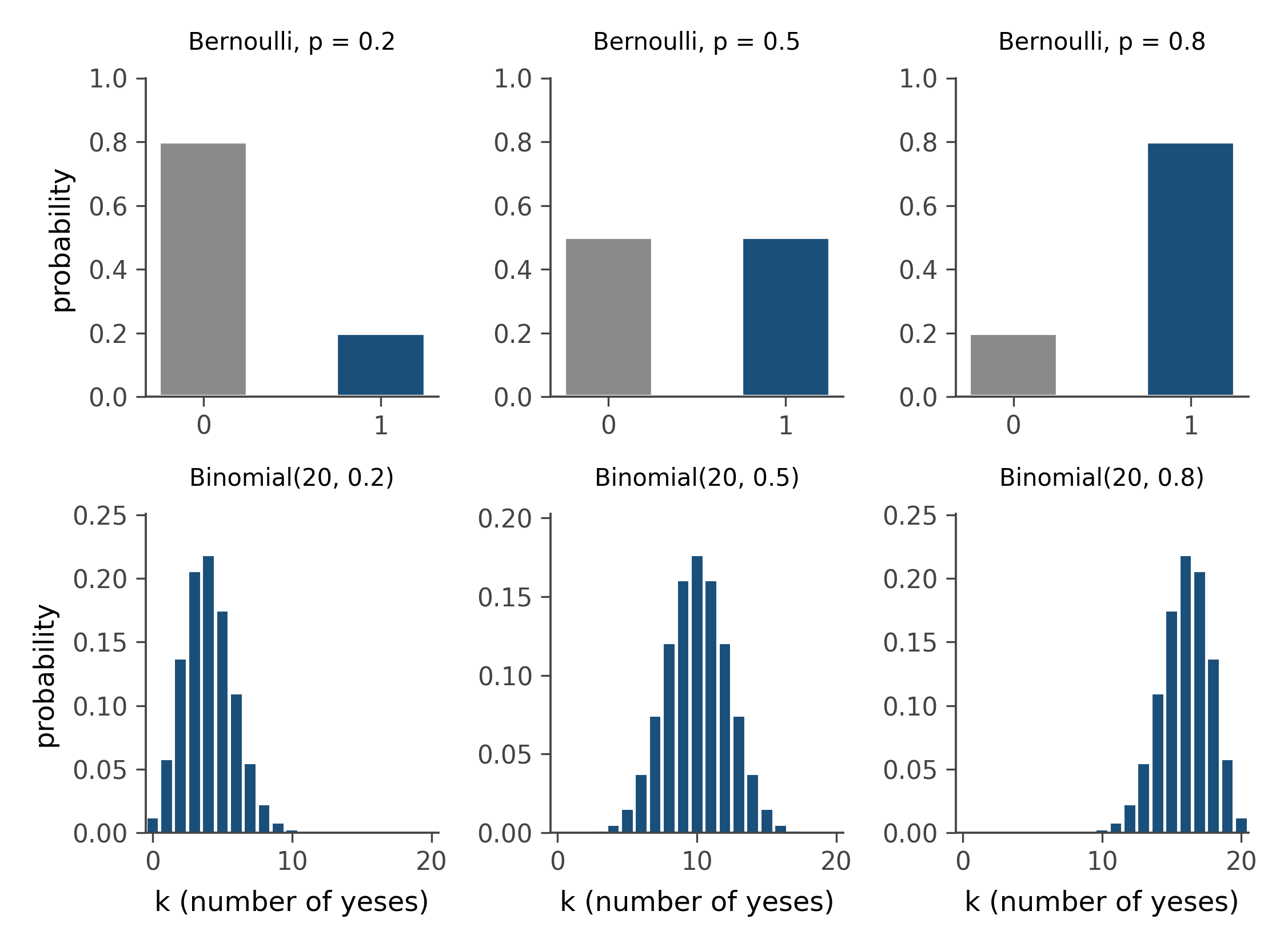
Where you meet binomials in the wild: anything counted from a fixed number of trials. Test scores out of 50. Free throws made in 10 attempts. People in a sample of 1,000 who report a given opinion. The story is always “fixed n, fixed p, count the yeses.”
6.3 Poisson: the rare event
A different story. You are not running a fixed number of trials; you are watching a clock or a region in space, and events happen at some average rate. Earthquakes per year above some magnitude. Cars arriving at a toll booth per minute. Typos per page. Cosmic rays striking your phone in an hour. Events are independent, the rate is approximately constant, and you count how many you observed in your window.
The distribution of that count is called Poisson, written Poisson(\lambda). Its single parameter \lambda is the average number of events expected in the window. Values live on the non-negative integers (0, 1, 2, …), with a characteristic shape that peaks near \lambda, drops off on both sides, and never quite reaches zero.
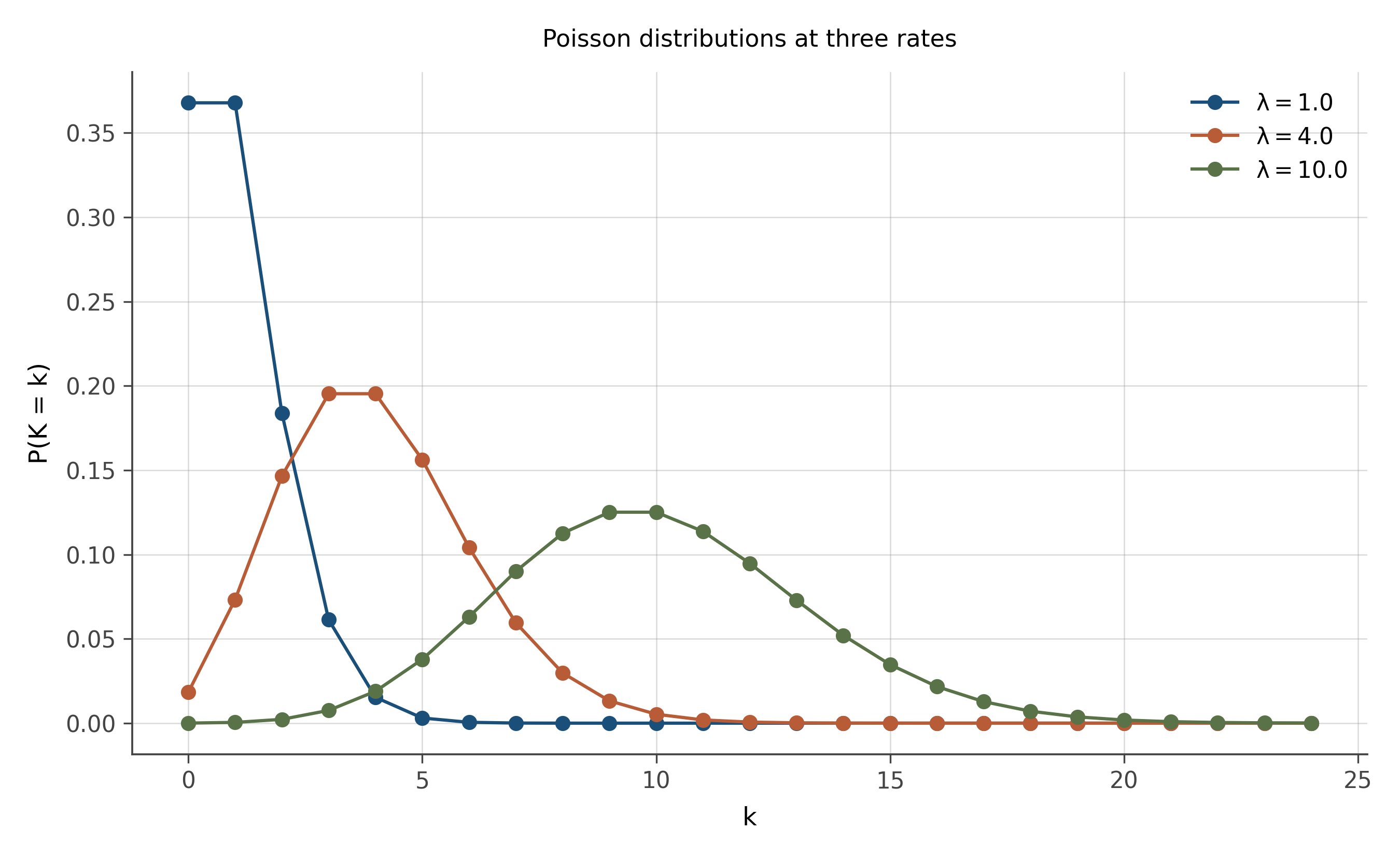
The Poisson story is the answer to “how many rare independent events in a fixed window?” When you see count data and the events are not all going to be yes-or-no with a fixed n, the Poisson is usually the right starting point. Many real count distributions are not exactly Poisson but are close enough that the Poisson is the right idealization.
A useful trick. If \lambda is large (say, more than 30), the Poisson starts to look like a normal distribution centered at \lambda with standard deviation \sqrt{\lambda}. This is a special case of a phenomenon we will spend chapter 14 working on.
6.4 Normal: the sum of many small things
The most important distribution in statistics, full stop. The bell curve. The Gaussian. The normal. There are reasons it shows up everywhere, and the reasons matter more than the formula.
The story: a normal distribution arises whenever the value you are measuring is the sum of many independent small contributions, none of which dominates the total. Human height is approximately normal because it is the sum of many small genetic and environmental influences. Measurement error is approximately normal because each measurement is a sum of many tiny independent perturbations. The mean of any sample (no matter what the underlying distribution is) is approximately normal once n is large enough. We will spend chapter 14 on that last fact, because it is the engine of inferential statistics.
A normal distribution is fully described by two numbers: its mean (where it is centered) and its standard deviation (how wide it is). The shape is symmetric about the mean, drops off rapidly on both sides, and has the characteristic 68-95-99.7 property: about 68% of the area is within one standard deviation of the mean, about 95% within two, about 99.7% within three.
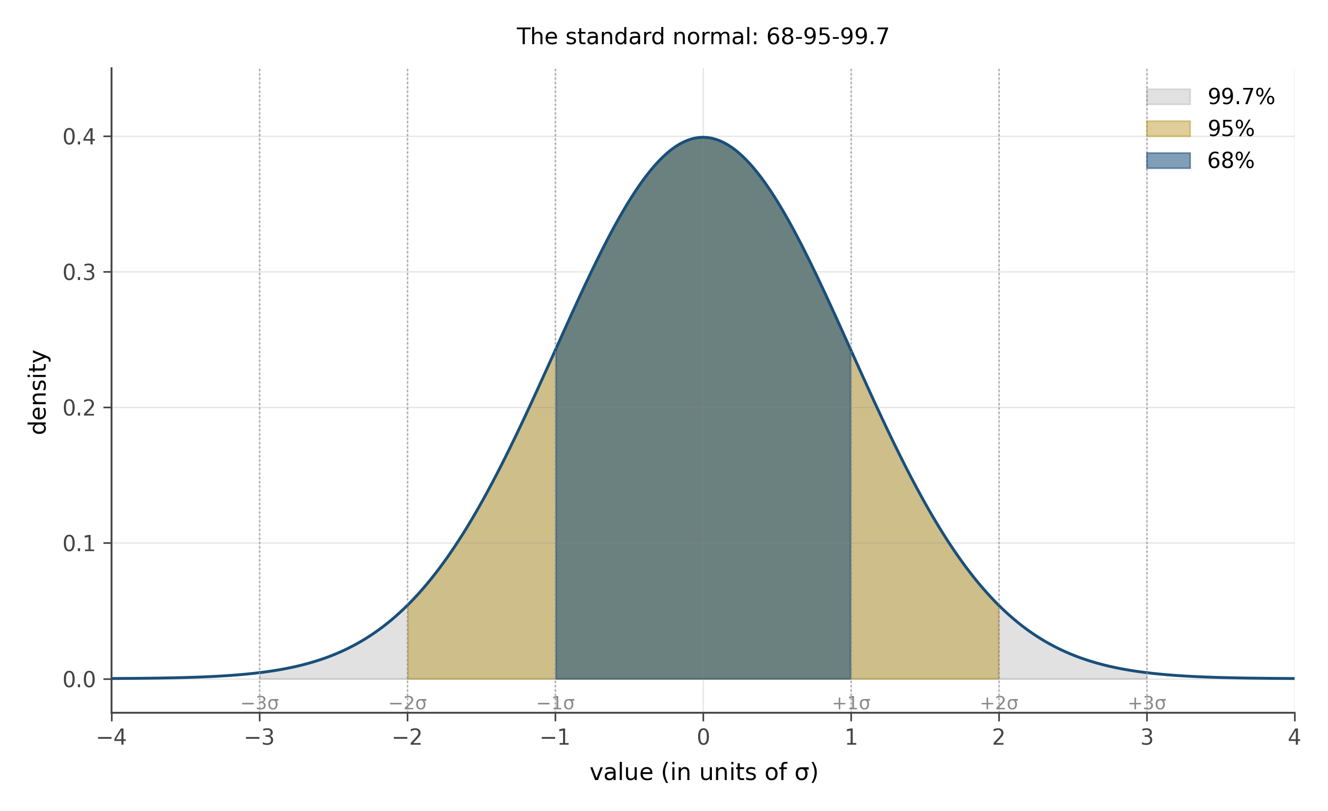
The 68-95-99.7 rule is worth memorizing. It lets you do quick sanity checks on any normal-shaped data: if a value is more than 2 sd from the mean, it is in the top or bottom 2.5% of the distribution. More than 3 sd, top or bottom 0.15%. The thresholds become natural after a few uses.
6.5 Exponential and log-normal: the wait, the multiplied
Two more shapes that recur, both heavy on the right side.
The exponential distribution is the story of waiting. You are watching for the next earthquake, the next bus, the next user click. Time elapses. The probability of waiting at least t more time units shrinks at a constant rate, regardless of how long you have already waited (the memoryless property). The distribution of the wait time has a peak at zero and a fast decay toward longer waits. Most waits are short, a few are surprisingly long. The single parameter is the rate \lambda, and the mean wait is 1/\lambda.
The log-normal distribution is the story of multiplied effects. Suppose a quantity is built up not by adding many small things but by multiplying them. The size of a city is roughly the product of historical advantages, each one acting as a multiplier. Income is roughly the product of skill, opportunity, market timing, and luck, each multiplying the previous. The log of such a quantity is a sum of small things, which (by the previous section’s story) is approximately normal. So the original quantity is the exponential of a normal, called log-normal.
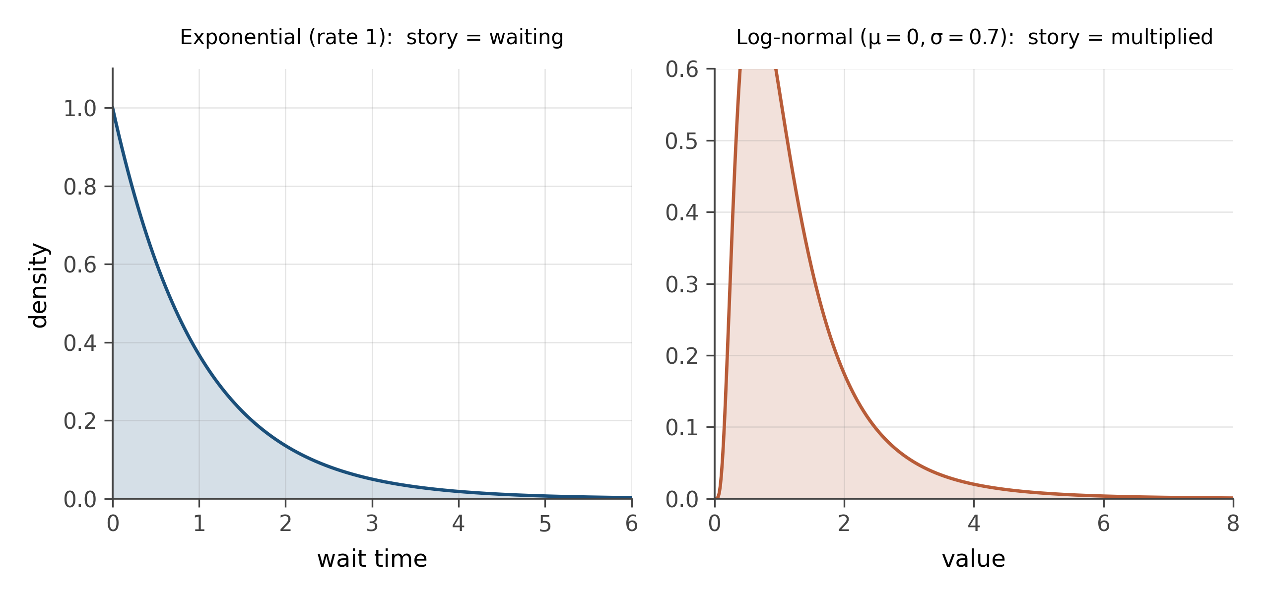
The first move when you see right-skew data is usually to take the log and see if the result looks normal. Often it does. Once it does, all the tools you have for working with normal distributions become available, applied on the log scale. Coefficients of regressions on log-transformed outcomes have a natural interpretation as percentage changes, which we will use heavily in the regression chapters.
6.6 The t: when n is small
One last shape. The Student’s t distribution, which looks almost like a normal but is not.
The story: when you compute the mean of a small sample, you do not actually know the population standard deviation; you have to estimate it from the data. That estimate has its own uncertainty, especially when the sample is small. The t distribution is the correct accounting for the extra uncertainty. It looks like a normal but with heavier tails, the heaviness controlled by a parameter called degrees of freedom that essentially equals the sample size minus one.
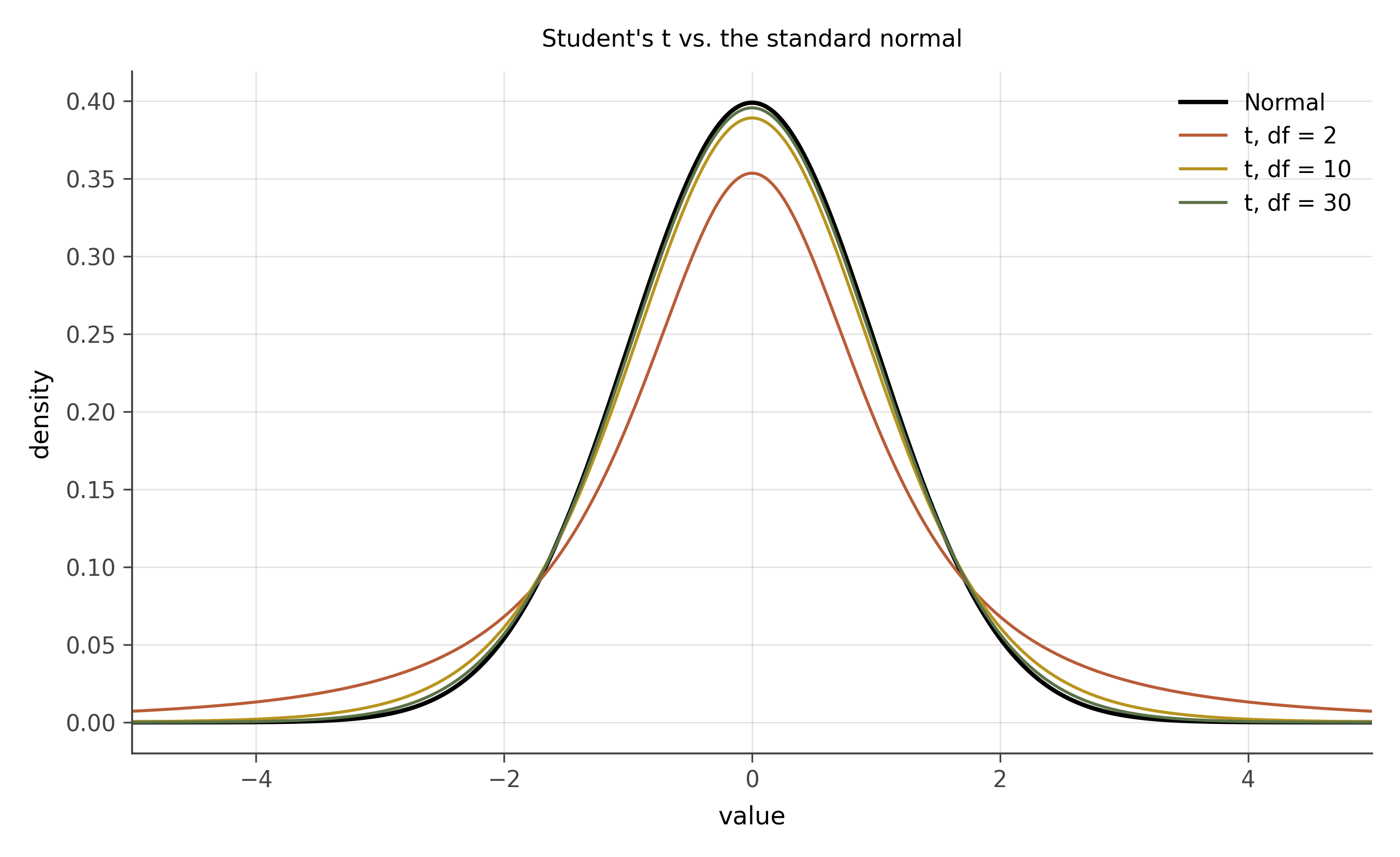
When the sample is large (say, n > 30), the t is indistinguishable from the normal. When the sample is small (say, n = 5), the t has noticeably fatter tails: more probability of extreme values, to account for the fact that the standard deviation estimate could itself be off. As n grows, the t converges to the normal.
You will meet the t the first time we do a confidence interval for a mean, in chapter 13. The reason hypothesis tests for small samples use the t and not the normal is exactly the story above.
Distributions are stories about generating processes. Six of them cover most of what you will see in working analysis: Bernoulli (yes-or-no), Binomial (counts of yeses), Poisson (rare events in a window), Normal (sums of many small things), Exponential and Log-normal (waits and products), and Student’s t (the normal’s small-sample cousin). Recognizing the story tells you which tool to use; the formulas come later.
Pick a column from any dataset you have access to, ideally something with at least a hundred values. Plot a histogram. Ask which of the six stories above best describes its shape. Then ask why: what process produced the values, and does that process match the story?
If the data is right-skewed, take the log and plot again. Does the log-transformed version look approximately normal? If yes, you have a log-normal column on your hands and a different set of tools applies.
A second prompt: pick two columns from the trade slice (exports_usd_millions and distance_km are good). Plot a histogram of each. Then plot a histogram of \log(\text{exports}) and \log(\text{distance}). Notice which transformation does meaningful work.
Each distribution in this chapter has a probability mass function (for discrete distributions) or probability density function (for continuous ones). The names attached to the formulas are sedimented history.
Jacob Bernoulli, working on games of chance in the late 1600s, gave his name to the simplest yes-or-no distribution. The binomial coefficient that appears inside Binomial(n, p) was studied earlier still, by Pascal and Fermat in their 1654 correspondence about gambling.
In 1837, Siméon Denis Poisson published a treatise on the probability of judicial verdicts that contained what we now call the Poisson distribution. Its earliest serious application was to the statistics of rare events in human populations: deaths from horse-kicks in the Prussian army, used by Bortkiewicz in 1898 as a textbook example.
The normal distribution was discovered three times. De Moivre derived it in 1733 as a limit of the binomial. Laplace developed it independently in 1810 inside what we now call the central limit theorem. Gauss arrived at it from a different direction in 1809, in his theory of measurement error. “Normal” as the popular name came only later, from Galton and Pearson at the end of the 1800s.
In 1908, a Guinness brewery statistician named William Sealy Gosset published the t distribution under the pen name Student, because his employer forbade publication under his real name. It is one of the most consequential pseudonyms in scientific history.
Log-normal and exponential are simpler in provenance: both fall out naturally once the normal exists and once you start thinking about waits and products.
Notation conventions across these distributions (Greek for parameters, Roman with hats for estimators) will be respected throughout the book. The hats become important in chapter 13, when we learn to estimate parameters from data.
Modern probability is much wider than the six distributions above. Three areas where the frontier is moving:
Heavy-tailed distributions and extreme value theory. Many real-world distributions (market returns, internet traffic, natural disasters) have tails far heavier than the normal predicts. The field of extreme value theory studies the maxima of random processes and provides distributions (Gumbel, Fréchet, Weibull) that are the right tools when the question is about rare extreme events rather than the bulk.
Distributions on networks and graphs. The “rectangle of rows and columns” assumption breaks down when the data is relational (who knows whom, who trades with whom). Modern probability has been extended to handle distributions on graphs, on permutations, on trees, on more exotic combinatorial objects. The recurring trade panel of this book is partly network data, and we will return to this in chapter 41.
Bayesian nonparametric models. When the right distribution is itself unknown, modern Bayesian methods place a prior over distributions themselves (Dirichlet processes, Gaussian processes), letting the data choose the right distributional family. This is one of the most active areas in current statistics and machine learning.
For now, the six stories cover everything in Parts One and Two of the book. The bigger zoo waits.
6.7 Practice problems
For each variable below, name the distribution that most likely describes it: number of phone calls received in an hour; height of adult women in cm; whether a coin lands heads; income in a country; time between earthquakes; number of children per family.
A distribution has a long right tail. You take the log; the result looks normal. What family of distributions is the original?
A Poisson distribution has \lambda = 6.4. What is the mean? Approximately what is the standard deviation? Why?
For Student’s t at df = 5, where do the tails sit relative to a standard normal? At df = 50?
Open the trade slice. Plot a histogram of
exports_usd_millions. Then plot a histogram of \log(\text{exports_usd_millions}). Which version is closer to a familiar shape from this chapter? What does that tell you about the underlying process?
- Why is “what process produced this data” a more useful question than “what is the formula”?
- Pick one distribution from the chapter. Explain its underlying story to a friend in three sentences.
- The mean of a sample becomes normal as n grows, no matter what the parent distribution looks like. Why is this almost magical?
Looking ahead
Chapter 4: The grammar of graphics. Now that you can recognize distributional shapes, the next chapter teaches the visual grammar that lets you communicate about them. Wilkinson’s three-layer grammar (data + aesthetics + geometry) plus the Cleveland-McGill perceptual hierarchy plus the discipline of small multiples. Continue →