8 Center, spread, shape – Pictures of Inference

8.1 Three numbers that summarize a column

You have a column of numbers. A million rows, maybe. You want to describe it in a way that fits in a sentence. What three numbers should you reach for?

The answer in most introductory courses is: the mean, the standard deviation, and not much else. That answer is not wrong. It is also not enough. A column of numbers is described well by three things: where it is centered, how spread out it is, and what shape it has. Each of these can be measured several ways, and the choice of measurement is itself a substantive decision.

The sections below lay out the choices. By the end of the chapter you will be reaching for the right one without thinking, and the words “mean” and “standard deviation” will sound, properly, like just one option among several.

8.2 Center: mean, median, mode

The mean is the arithmetic average. Sum the values, divide by the count. It has a clean physical interpretation: if you put each data value as a unit weight on a number line, the mean is the point where the line balances.

The median is the middle value when the data are sorted. Half the values fall below it, half above. It has a different physical interpretation: it is the point that minimizes the sum of absolute distances to the data.

The mode is the most common value, or for continuous data, the value where the distribution peaks.

For perfectly symmetric distributions, all three are equal. For skewed distributions, they pull apart. The mean chases the long tail. The median ignores it. The mode plants itself at the peak.

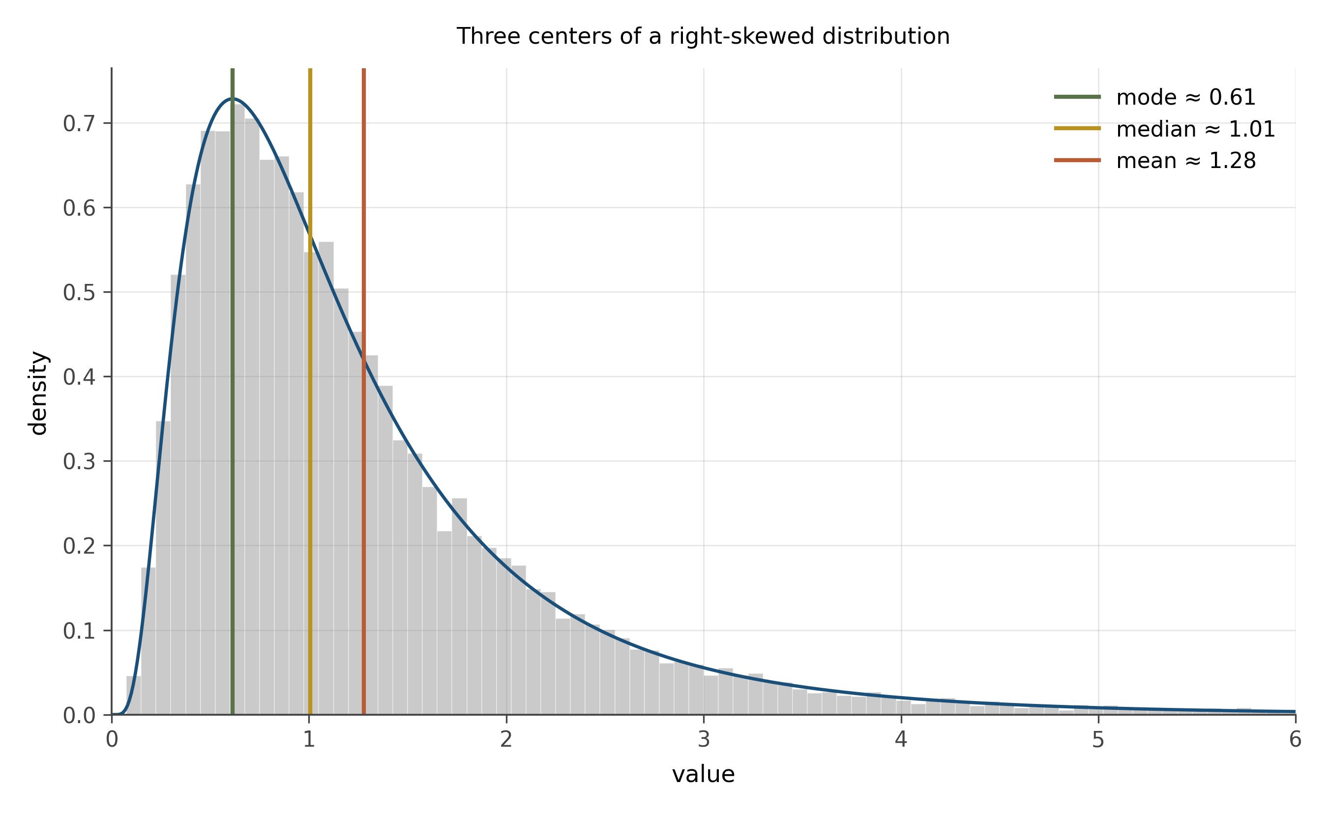
Figure 8.1: A right-skewed distribution (log-normal-shaped) with the three centers marked. The mode sits at the peak, the median sits to its right (because more than half the area is to the right of the mode), and the mean sits even further right (because the long tail pulls the balance point that way). For symmetric distributions, all three coincide.

Income is the canonical example. A small number of very high earners pull the mean far above the median. The median household income in a country can be $50,000 while the mean is $80,000, simply because a tiny fraction of the population earns enough to drag the average up. When a journalist wants to make inequality look mild, they report the mean. When they want to make it visible, they report the median. Both numbers are correct. The choice of which to report is a choice about what story to tell.

The general rule. For symmetric data, mean and median agree, and the mean is more efficient (uses more of the data). For skewed data, the median is the more honest summary of “what does a typical observation look like.” The mean is still useful, but it tells you about the aggregate (the total divided by the count), not about the typical.

8.3 Spread: range, variance, sd, IQR

A column with mean 50 could have all its values within a millimeter of 50, or it could have half its values at 0 and half at 100. The mean is the same. The spread is wildly different.

Several ways to measure spread.

The range is the largest value minus the smallest. Easy to compute. Almost useless: a single outlier can blow the range up. Don’t use it for anything serious.

The variance is the average of squared deviations from the mean,

s^2 = \frac{1}{n-1} \sum_{i=1}^n (x_i - \bar{x})^2.

The squaring matters. It prevents positive and negative deviations from cancelling, and it weights large deviations more heavily than small ones. Variance has the wrong units for direct interpretation (squared whatever-the-data-was-in), so we usually report its square root, the standard deviation s. Compare s to the mean to get a sense of relative spread.

The interquartile range, or IQR, is the spread between the 25th percentile and the 75th percentile. Middle half of the data, as a single number. By ignoring the top and bottom 25%, the IQR becomes robust to outliers in a way the standard deviation is not.

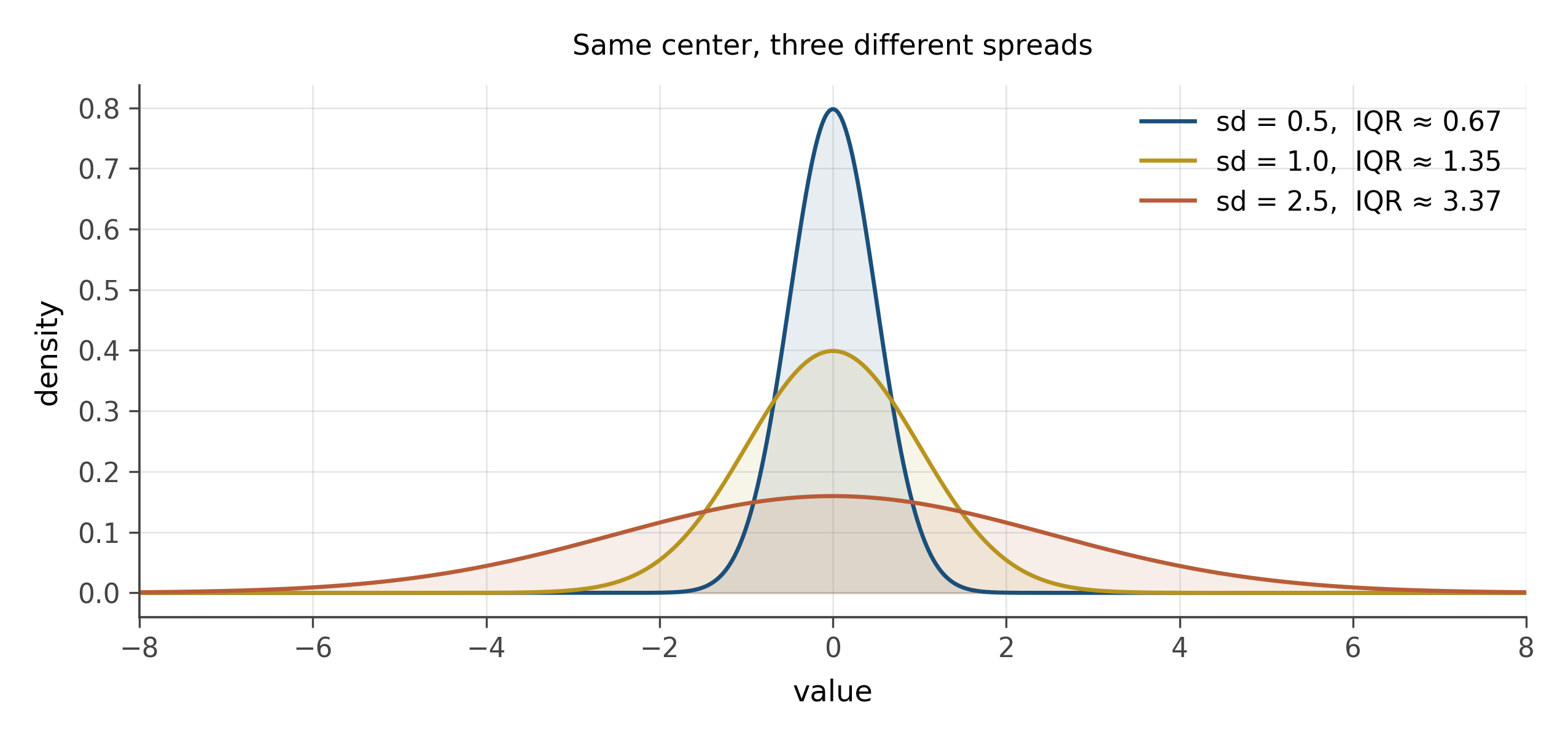
Figure 8.2: Three distributions with the same mean but very different spreads. The left has standard deviation 0.5; the middle has 1.0; the right has 2.5. The IQR ratios track the standard deviation ratios because the data is normal-shaped. For non-normal data, the two measures can diverge sharply.

When the data is approximately normal, the standard deviation is the right tool. The 68-95-99.7 rule from chapter 3 tells you exactly how to interpret it. When the data is skewed or has outliers, the IQR is usually more honest, because the standard deviation can be inflated by a few extreme values that are not representative of the bulk.

8.4 Shape: skewness and kurtosis without the formulas

Beyond center and spread, distributions have shape.

Skewness measures asymmetry. A right-skewed distribution has a long tail on the right (income, file sizes, earthquake magnitudes). A left-skewed distribution has a long tail on the left (less common; one example is age at death in low-mortality populations). A symmetric distribution has zero skewness.

Kurtosis measures tailedness, roughly speaking. A high-kurtosis distribution has heavier tails than a normal: more probability of extreme values. A low-kurtosis distribution has lighter tails. Financial returns famously have high kurtosis: extreme moves are more common than a normal distribution would predict, and the difference matters for risk management.

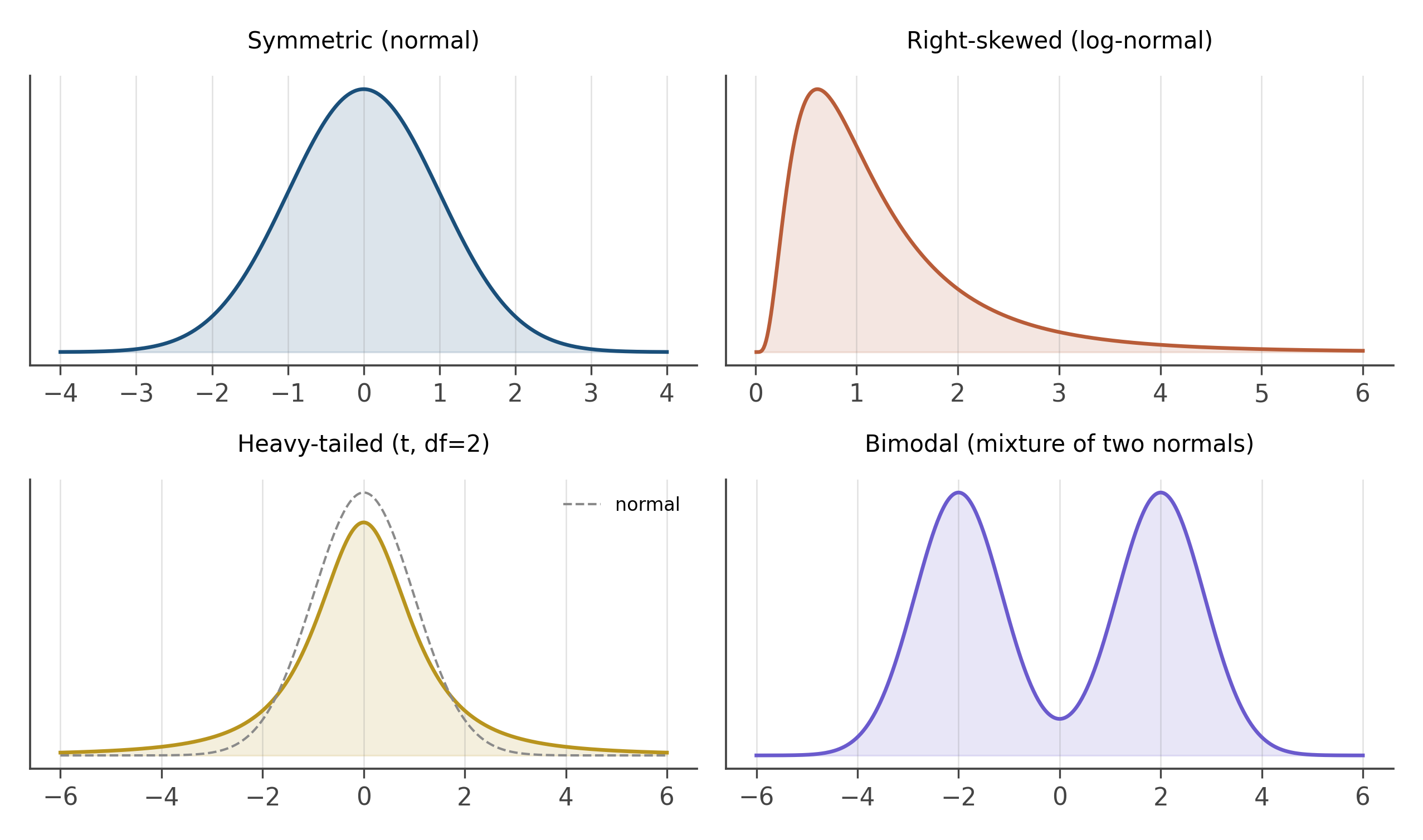
Figure 8.3: Four shapes that recur: a roughly symmetric (normal) distribution, a right-skewed (log-normal) distribution, a heavy-tailed (Student’s t with low df) distribution, and a bimodal distribution. Knowing the formulas for skewness and kurtosis matters less than recognizing the shapes.

The numerical formulas for skewness and kurtosis exist and you can look them up. Knowing the formulas matters less than recognizing the shapes. When you look at a histogram, your first move is: symmetric or skewed? Light-tailed or heavy-tailed? One peak or several? Those four binary questions catch most of the shape information you need for early-stage analysis.

Bimodal distributions deserve special mention. When a distribution has two peaks, the mean and median are both potentially meaningless: they fall in the valley between the peaks, where almost no actual observations live. Bimodality is usually a sign that two different processes have been pooled together: men and women, treated and control, before and after. The right move when you see bimodality is to find the splitting variable and disaggregate.

8.5 Robustness: what an outlier does

An outlier is an observation that lies far from the bulk. The word does no semantic work; it is just a description of distance from the center.

The mean and standard deviation are not robust to outliers. A single extreme value can change them substantially. The median and IQR are robust. A single extreme value barely moves them at all.

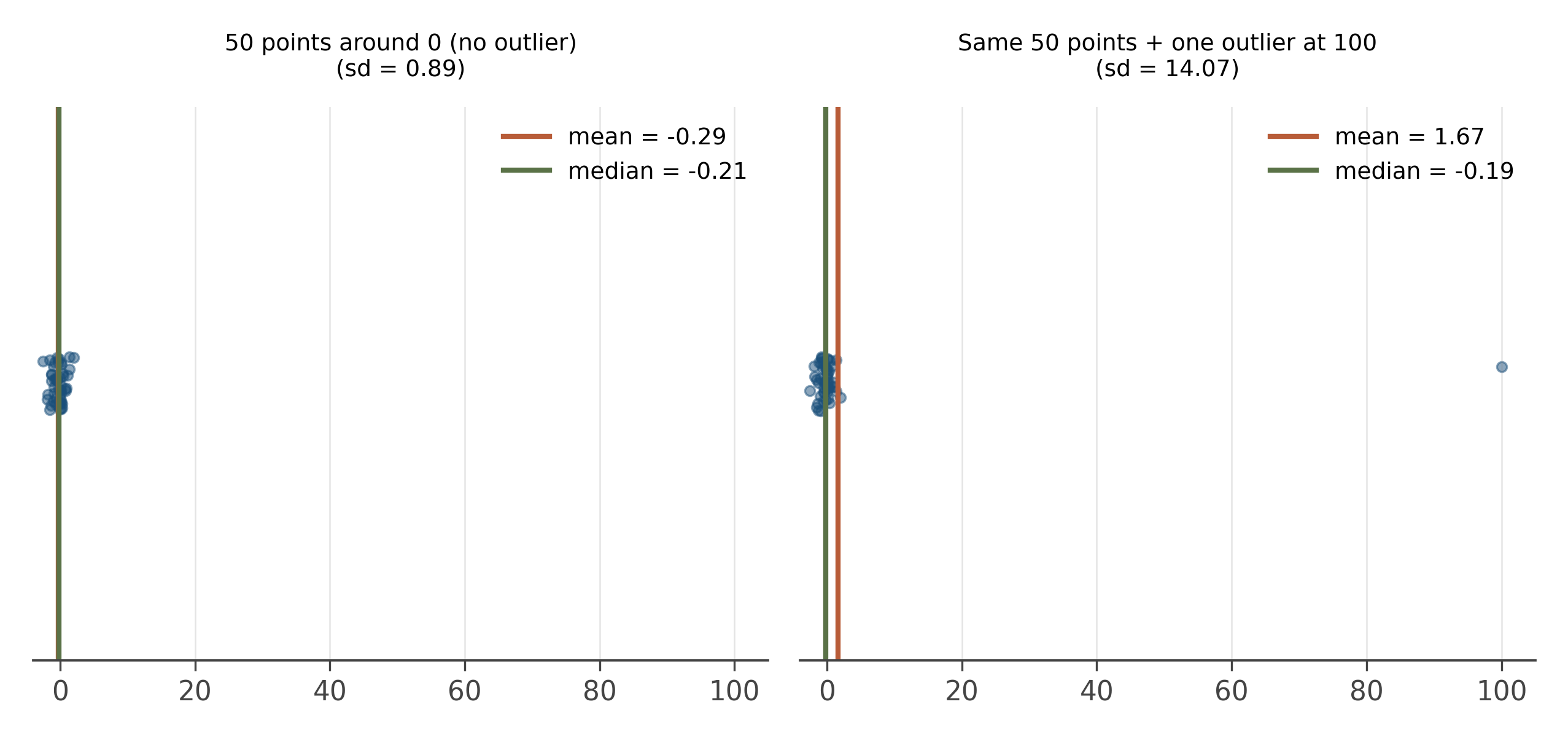
Figure 8.4: Fifty points sampled near zero, with one extreme outlier added at 100. The mean is dragged toward the outlier, while the median barely moves. The standard deviation explodes; the IQR holds steady. Robustness is the difference between summary statistics that lie about an outlier and summary statistics that ignore it.

The robustness distinction is more important than it sounds. Real datasets have outliers. Sometimes those outliers are real (a billionaire in an income survey). Sometimes they are errors (a typo, a unit confusion, a sensor malfunction). In both cases, summary statistics that are pulled around by the outliers will mislead. Robust statistics give you a stable summary of the bulk, which is usually what you want before you have figured out whether the outliers should be kept.

Use the median and IQR when you do not yet know what your outliers are. Use the mean and standard deviation when the data is approximately normal and you are confident the outliers are real and meaningful.

8.6 The five-number summary and the boxplot

A compact summary captures center, spread, and outliers in five numbers: the minimum, the 25th percentile, the median, the 75th percentile, and the maximum. Tukey called this the five-number summary, and it is one of the most useful descriptive tools in the discipline.

The boxplot is the visualization of the five-number summary. A box from the 25th to the 75th percentile, a line at the median, whiskers extending to the most extreme non-outlier values, and individual points for outliers beyond the whiskers (typically beyond 1.5 IQRs).

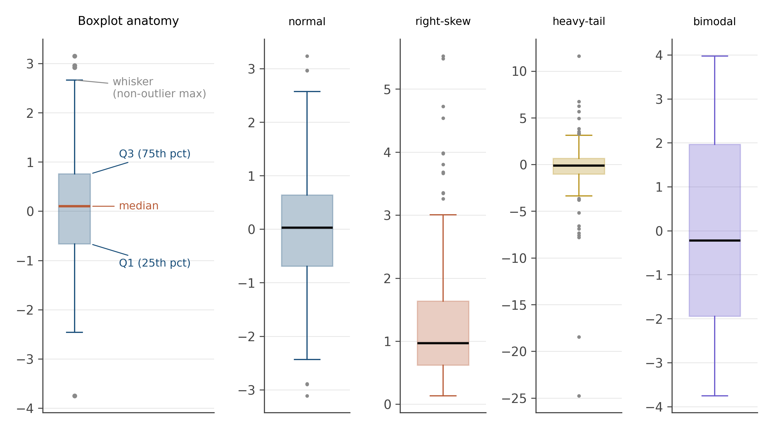
Figure 8.5: Anatomy of a boxplot, alongside boxplots for the four shapes from earlier in the chapter. Boxplots are excellent for comparing distributions across groups: row of boxplots, one per group, is often the right first chart. They hide the within-box shape, which is why a bimodal distribution and a uniform distribution can have similar boxplots.

Boxplots are the right summary visualization for many comparisons across groups: trade flows by year, test scores by class, response times by condition. They show center and spread and outliers in a small footprint, which makes them ideal for small multiples. A row of boxplots, one per group, is often the right first chart for any cross-group comparison.

Their weakness: they hide the shape of the distribution within the box. A bimodal distribution and a uniform distribution can have the same boxplot. When shape matters, a violin plot (which adds a kernel density estimate to each side of the box) is the better choice. We will meet violin plots formally in chapter seven.

Key insight

A column of numbers wants three things named: where it is centered, how spread out it is, and what shape it has. Each can be measured several ways, and the right choice depends on whether the data is symmetric, whether outliers are present, and what story the summary needs to tell. Robust statistics (median, IQR) are the default when you do not yet know your data; classical statistics (mean, sd) come into their own when the data is approximately normal.

Try this

Open the bilateral trade panel. For the exports_usd_millions column, compute: mean, median, standard deviation, IQR, and the five-number summary. Plot a histogram and a boxplot.

Which summary best describes the column? If you had to give one number to a journalist who wanted to know “how much typical bilateral trade is between these countries,” which would you give?

Then take the log of exports_usd_millions and recompute. Notice which summary changes most dramatically and which barely changes. The answer tells you something about the underlying distribution and about robustness, both at once.

Inside the math: where the n-1 comes from

The variance formula has n-1 in the denominator, not n. This is Bessel’s correction, and the reason for it is one of the cleanest derivations in statistics.

When you estimate the population variance from a sample, you use the sample mean \bar{x} in place of the unknown population mean \mu. The sample mean minimizes \sum(x_i - c)^2 over choices of c, which means \sum(x_i - \bar{x})^2 is systematically smaller than \sum(x_i - \mu)^2 would have been. Dividing by n would therefore underestimate the population variance.

The correction is exactly n/(n-1): dividing by n-1 instead of n produces an unbiased estimator of the population variance. The intuition is that we have used up “one degree of freedom” in estimating the mean from the same data, so the effective sample size for estimating spread is n-1 rather than n.

This shows up everywhere in inferential statistics. Whenever you see n-1 in a denominator, look for an estimated mean somewhere in the numerator. Degrees of freedom are the bookkeeping system for this correction, and we will encounter them again in the t distribution (chapter 13), in regression (chapter 16), and in everything that follows.

Frontier note

Robust statistics is a substantial sub-field of modern statistics. Beyond the median and IQR, there are robust analogues of almost every classical procedure: M-estimators, trimmed means, winsorized means, the median absolute deviation (MAD), Huber regression, and many more. The frontier work is in high-dimensional robustness: when the data has thousands of variables, classical procedures break down in ways that simple median-and-IQR replacements do not fix.

In modern empirical economics, the practice of reporting both classical and robust summaries (or robust standard errors, which we will meet in chapter 34) is now standard for any serious paper. The reason is partly the credibility revolution and partly the recognition that real economic data has fat tails, outliers, and clusters, and pretending otherwise produces fragile inference.

8.7 Practice problems

Compute by hand: mean, median, mode, range, variance, sd, IQR, and the five-number summary for the values \{1, 3, 3, 5, 7, 8, 9, 12, 100\}.
Which summary statistic from the previous problem changes the most if you remove the 100? Which barely changes? What does that tell you about robustness?
A distribution has skewness +2. What does that tell you about the shape? What if the skewness is -2?
A boxplot shows three distributions side by side. Without seeing histograms, which features can you compare confidently? Which would you want histograms for?
Open the trade slice. Compute the mean and the median of exports_usd_millions. Which is larger? Why? Which would you report to a journalist?

Reflect before moving on

Mean and median tell you different things. Pick a real-world quantity where you would report the median over the mean. Explain.
The IQR ignores the top and bottom 25%. What information are you giving up by reporting it instead of the standard deviation?
The bimodality warning sign comes up again and again. Why is bimodality usually a clue to disaggregate?

Looking ahead

Chapter 6: Lying with charts. Summary statistics are powerful, which means they can deceive. The next chapter catalogs the five most common visual lies (truncated axes, cherry-picked windows, area distortion, dual axes, log scales muting growth) and the honest defaults that prevent them. Continue →