13 Reading tables
- The anatomy of a regression table
- What summary statistics tables hide and reveal
- Balance tables as a window into randomization quality
- The crimes that show up in published tables
13.1 A table is a chart with words
A table is a chart. Its geometry is a grid of cells, its aesthetic mappings are row-position and column-position, and its data values are typed into the cells. The same questions you ask of a chart (what is the data, what is the encoding, what is the geometry) apply to a table, and the same critical-reading skill that lets you spot a misleading chart lets you spot a misleading table.
This chapter walks through three common kinds of tables you will meet in research papers: regression tables, summary statistics tables, and balance tables. Each has conventions. Each has crimes. Knowing both lets you read papers with comprehension instead of glaze.
13.2 Anatomy of a regression table
A regression table reports the results of one or several regression models. Conventionally, each column is a different model specification, and each row is one variable’s coefficient. Standard errors appear in parentheses below each coefficient. Stars mark statistical significance at conventional thresholds, though the convention varies by journal.
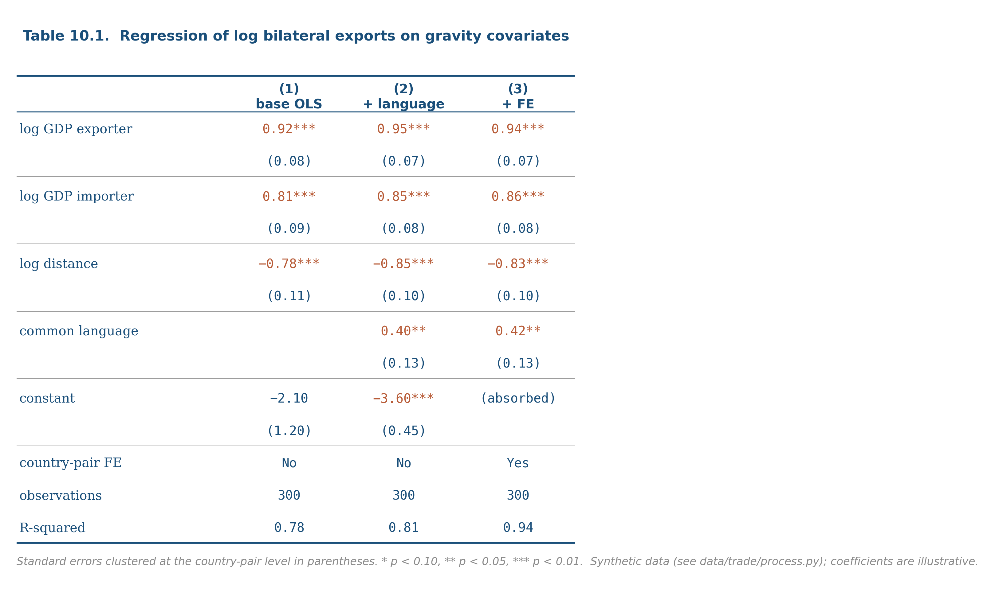
Reading from the top down:
Column headers identify each model. Sometimes “(1)”, “(2)”, “(3)” or short descriptions (“OLS”, “with FE”, “with controls”).
Row labels identify each regressor. The reference group of any categorical variable is omitted; its effect is absorbed into the intercept.
Coefficient cells show the point estimate. Standard errors appear in parentheses below, sometimes in brackets if a different uncertainty quantity (confidence interval, t-statistic) is being shown. Stars (, , ) mark statistical significance at conventional thresholds.
Bottom rows report sample-level diagnostics: number of observations, R-squared (for OLS), F-statistic, fixed-effects indicators (“Yes” or “No”), clustering indicators, and any other model-level metadata.
The crimes that show up in regression tables:
- Star-only reading. A coefficient that crosses the 0.05 threshold gets a star; one that misses by a tenth gets nothing. Readers who skim by stars misjudge the strength of evidence.
- Specification-switching without comment. Going from column 1 to column 2, the coefficient on the variable of interest moves dramatically. The author does not discuss why. The reader is supposed to assume the new specification is correct.
- Decimal mismatch. Some coefficients reported to four decimals, others to one. The mix usually hides where the action is.
- Hidden controls. “Controls included” with no list of what.
The defensive move on a regression table is to read across columns first, looking for stability. The coefficients of interest should not bounce around as you add or drop covariates. If they do, the model is fragile and the headline finding is suspicious.
13.3 Summary statistics tables
A summary statistics table describes the dataset before any analysis. Each row is one variable; each column is a summary statistic (mean, sd, min, max, percentiles). The table is the dataset’s introduction, and a careful reader spends real time on it.
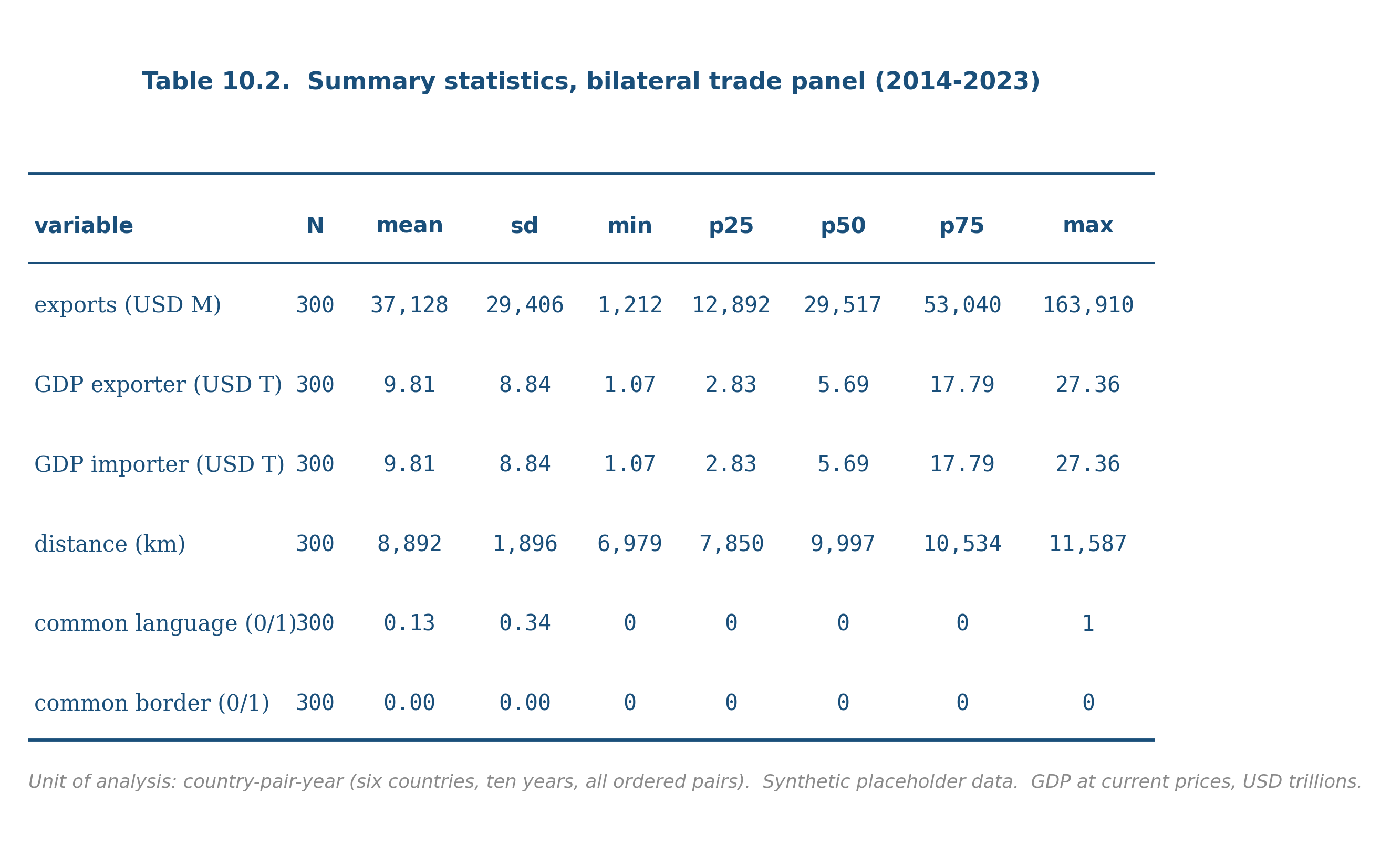
The questions to ask:
- What is the unit of analysis? Is each row in the underlying data a country-year, a person, a transaction?
- What are the units of each variable? USD, percent, count, log-transformed?
- Are the missing observations counted? If a variable has 1,000 observations and another has 800, where did the 200 go?
- Are the summary statistics weighted? Survey data with sampling weights is summarized differently from raw data.
- Are there outliers driving the means? If the mean is far from the median, the distribution is skewed and the mean is not the typical value.
A good summary statistics table answers all of these implicitly through its structure and its footnotes. A bad one buries them.
13.4 Balance tables
A balance table is the dataset-description chapter for randomized experiments and quasi-experimental designs. Each row is a covariate; columns show the mean of that covariate within the treatment group, the control group, the difference, and a p-value for the difference.
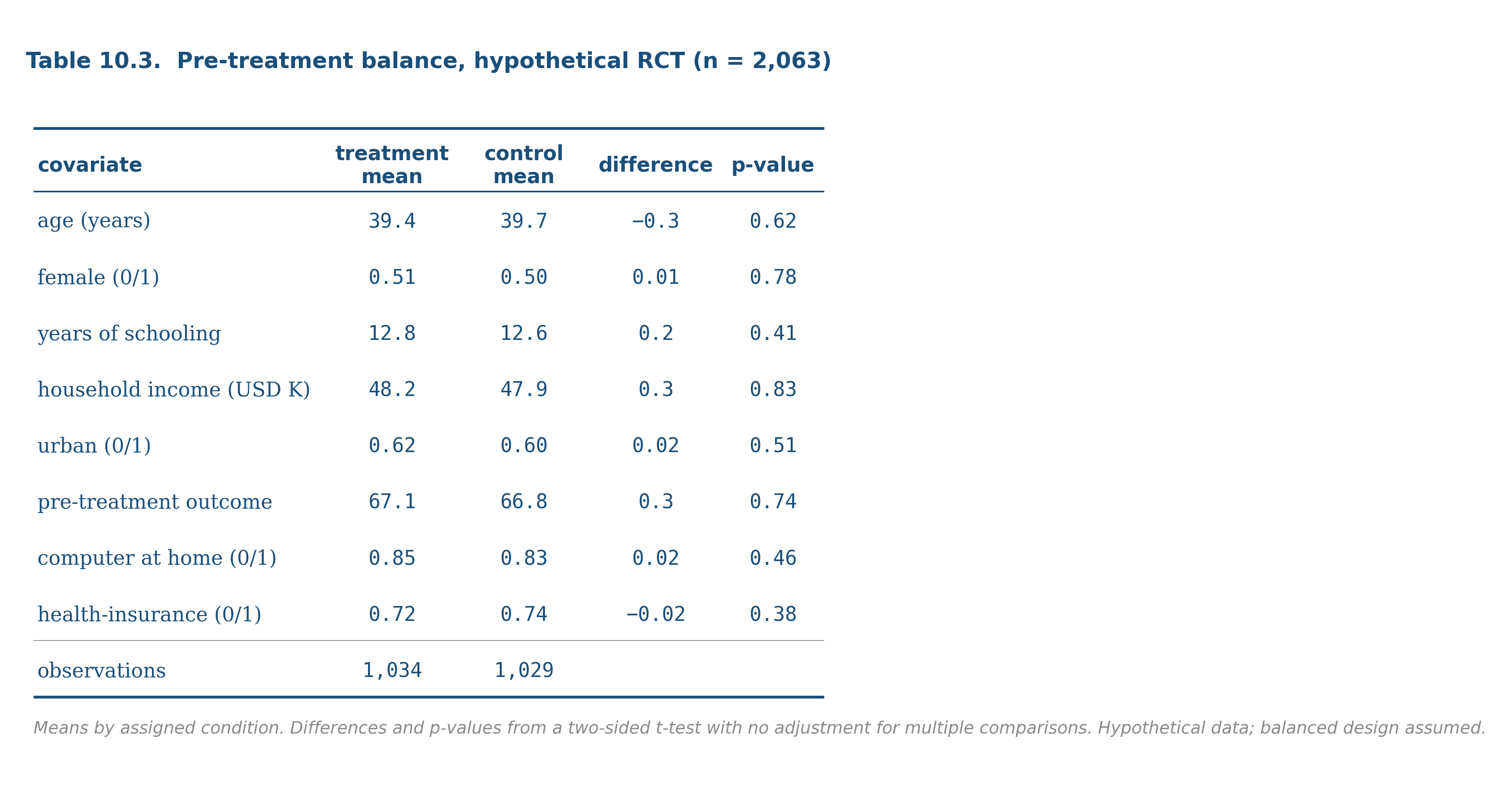
The visual story is whether the treatment and control groups look comparable on observable characteristics. A well-randomized experiment produces a balance table where most of the differences are small and the p-values are scattered uniformly between 0 and 1. A balance table where many differences are large or many p-values are small is a red flag: either the randomization failed, the design is observational rather than experimental, or there is selection at play.
For quasi-experimental designs (DiD, RD, IV), the balance table is more complicated but plays the same role: are the comparison groups similar on observables, conditional on the design’s assumptions?
The defensive move on a balance table is to count the variables and the p-values. Out of N tests, you would expect about N/20 to be significant at the 0.05 level by chance alone. If the share is dramatically higher, ask why.
13.5 What every table needs and what most do not
Three things every well-made table has:
- A title that names the dataset and the unit of analysis. “Regression of log exports on gravity covariates, country-pair-year level, 2014-2023.”
- A note that names the standard errors. “Standard errors clustered at the country-pair level.”
- Units and signs that match the prose. If the regressor is “log GDP” the coefficient is an elasticity; the prose should call it that.
Three things most published tables omit:
- Counts of the actual observations used. “N = 1,247” says how many rows survived the model’s exclusions. Many tables hide this.
- Comparison to a benchmark. If the gravity coefficient on log GDP is 0.95 and the literature averages 0.9, a reader needs to know.
- A footnote explaining outliers and exclusions. If the regression dropped country-years with exports below $100,000, say so.
These omissions are not malicious in most cases; they are conventions. The reader’s job is to read past the conventions and reconstruct what was actually done.
A table is a chart with words. The same critical-reading skill that catches misleading charts catches misleading tables. Read regression tables across columns first, looking for stability. Read summary tables for unit-of-analysis and unit-of-measurement. Read balance tables for the share of significant differences relative to what chance would produce. The defensive move is always the same: do not skim, decompose.
Find one regression table in a paper from your field. Apply the four-crime checklist:
- Are the coefficients on the variable of interest stable across columns?
- Is the coefficient reading sensitive to the stars, or do you read the magnitudes and uncertainties directly?
- Are the decimal places consistent across rows?
- Are the controls listed by name, or just “controls included”?
Then summarize, in three sentences, what the table actually shows. If you cannot do that without going back to the prose, the table is failing at its job.
The footnote “Standard errors clustered at the country-pair level” is doing more work than most readers realize.
Default OLS standard errors assume the regression residuals are independent across observations. When observations are grouped (by country, school, household, time period) and the residuals within a group are correlated with each other, default standard errors are too small, sometimes by orders of magnitude. The fix is cluster-robust standard errors, which adjust for the within-group correlation.
The choice of clustering level is substantive. Cluster too narrowly and you fail to capture the real correlation. Cluster too broadly and you lose statistical power. The wrong choice can either make a real effect look insignificant or make a noisy effect look significant.
Modern best practice in empirical work is to cluster at the level of treatment assignment (or the level of the natural unit, when the design is observational), and to report robustness to alternative clustering choices. The footnote is the quietest line in the table and one of the most important.
- A table footnote saying “robust standard errors clustered at the firm level” looked like fine print to you a year ago. What does it mean to you now? What did you have to learn to read it?
- The chapter argued that hidden controls are a crime. Why? What is the reader losing when “controls included” is the only documentation?
- Regression tables are the single most common quantitative artifact in published research. Why do most readers skim them? What would change if everyone read them carefully?
The credibility revolution in empirical economics has tightened table conventions over the last fifteen years. Three trends worth knowing:
Coefficient plots replacing tables. Many modern papers in causal inference now show coefficient plots in the body of the paper and relegate the full tables to the appendix. The visual chapter (chapter 8) made the case for why this is an improvement.
Pre-registration and open code. When the analysis code is published alongside the paper, the table is no longer the final word; it is one of many possible summaries the reader could compute themselves. This dilutes the rhetorical power of any particular table while improving the credibility of the overall finding.
Specification curves. Instead of two or three columns of a regression table, modern robustness checks display the distribution of estimates across many defensible specifications. Simonsohn, Simmons, and Nelson’s “specification curve analysis” is one widely-cited version. The visual move is from “here are three models I chose” to “here is what the entire defensible model space looks like.”
The general direction: less reduction, more transparency. Tables are still useful but they are no longer the only thing.
13.6 Practice problems
Find a regression table in a recent paper. Identify the dependent variable, the variable of interest, the control variables, and the standard-error specification.
The same table reports R-squared = 0.04 in column 1 and R-squared = 0.78 in column 4. What changed between the two columns? What does the change tell you?
A balance table for an experiment shows 20 covariates, of which 4 have p < 0.05 differences between treatment and control. Is this evidence of failed randomization, or is it consistent with chance? Compute.
A summary statistics table reports a variable with mean 50,000, median 32,000, and max 4,500,000. Sketch the implied distribution. What family from chapter 3 fits best? What summary would you report instead of the mean?
Take any table from a paper you respect and re-render it as a coefficient plot or a small-multiples chart. Decide which version is more informative.
Looking ahead
End of Part I. The skills the part has built (data structure, probability, distributions, visualization, summarization, critical reading, mathematical literacy, table literacy) are the foundation for Part II, where you will use them to do an actual analysis end to end. Part II is being drafted; chapter 11 (the empirical paper, walked through) is the planned capstone for Part I and is in the queue.