14 Workbook · Distributions in the wild
- Recognizing distributional shape from a histogram alone
- Matching shape to a process-level story
- Applying the 68-95-99.7 rule and the log-transform reflex
Eight histograms follow. For each one, your task is to name the shape, identify the underlying process from the chapter-3 story catalog, and answer one or two specific quantitative questions. Solutions are hidden behind a click. Resist looking until you have written your answer down.
The skill is shape-to-story matching. Working analysts do this in five seconds when they see new data. By the end of this workbook you should be doing it too.
14.1 Warmups
14.1.1 Problem 1: Adult heights
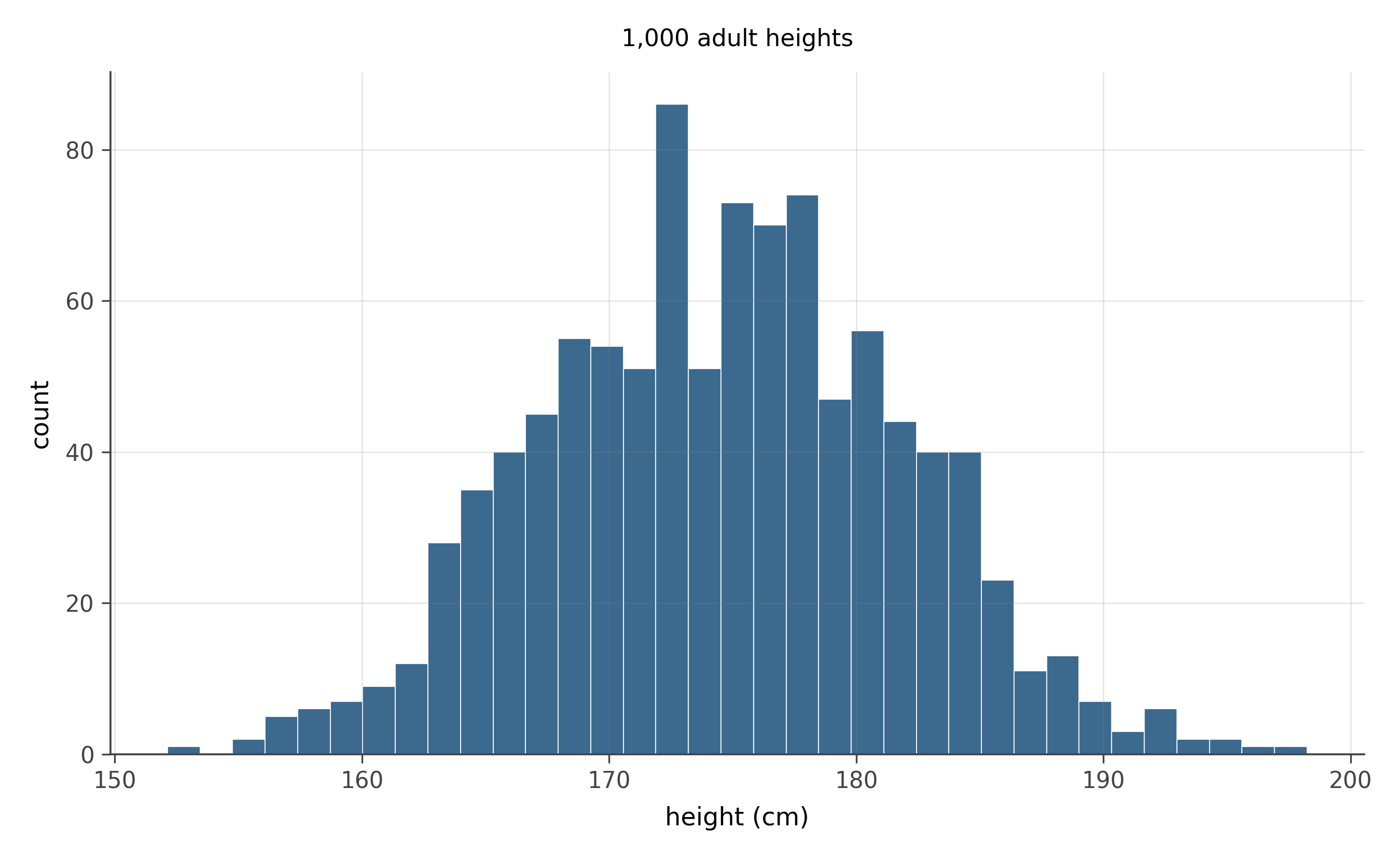
Without computing anything:
- What shape best describes this distribution?
- What chapter-3 story produces this shape?
- If the mean is 175 cm and the standard deviation is 7 cm, where do approximately 95% of the values fall?
Shape. Approximately normal. Symmetric, single peak, smooth decay on both sides, no long tails.
Story. “Sum of many small independent contributions.” Adult height is shaped by many genetic and environmental influences, none of which dominates the total. The central limit theorem applies and the result is approximately normal.
95% rule. By the 68-95-99.7 rule, about 95% of the values fall within 2 standard deviations of the mean. With \bar{x} = 175 and s = 7, that interval is 175 \pm 2(7) = 175 \pm 14 cm, or roughly 161 to 189 cm.
14.1.2 Problem 2: Bus stop wait times
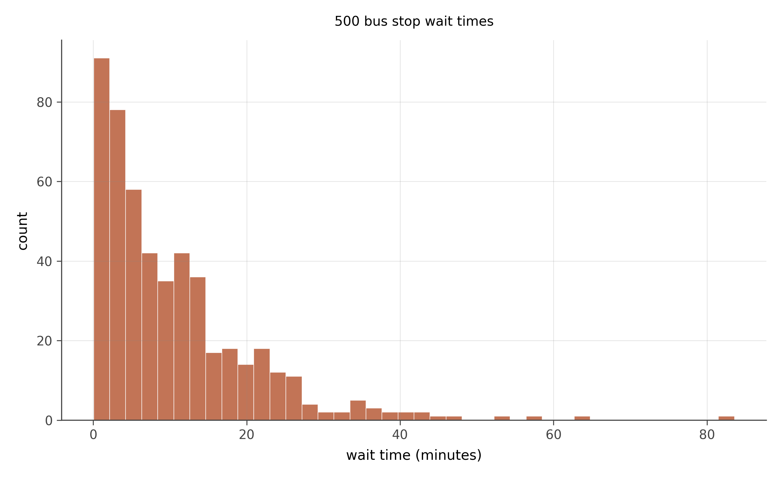
- What shape?
- What story produces it?
- Is the mean larger or smaller than the median? Why?
- If the mean wait is 10 minutes, what is the probability of waiting more than 20?
Shape. Exponential. Peak at zero, fast decay to the right, no negative values.
Story. “Memoryless waiting.” Events (bus arrivals) happen at a constant rate; the time until the next one is exponentially distributed with rate \lambda.
Mean vs. median. Mean is larger than median because the distribution is right-skewed. For an exponential with rate \lambda, the mean is 1/\lambda and the median is \ln(2)/\lambda \approx 0.693/\lambda. The median is roughly 70% of the mean. So a mean wait of 10 minutes implies a median around 7.
P(X > 20). With mean 10, the rate is \lambda = 1/10 = 0.1. The exponential survival function gives P(X > 20) = e^{-\lambda \cdot 20} = e^{-2} \approx 0.135, or about 13.5%.
14.2 Core problems
14.2.1 Problem 3: Typos per page
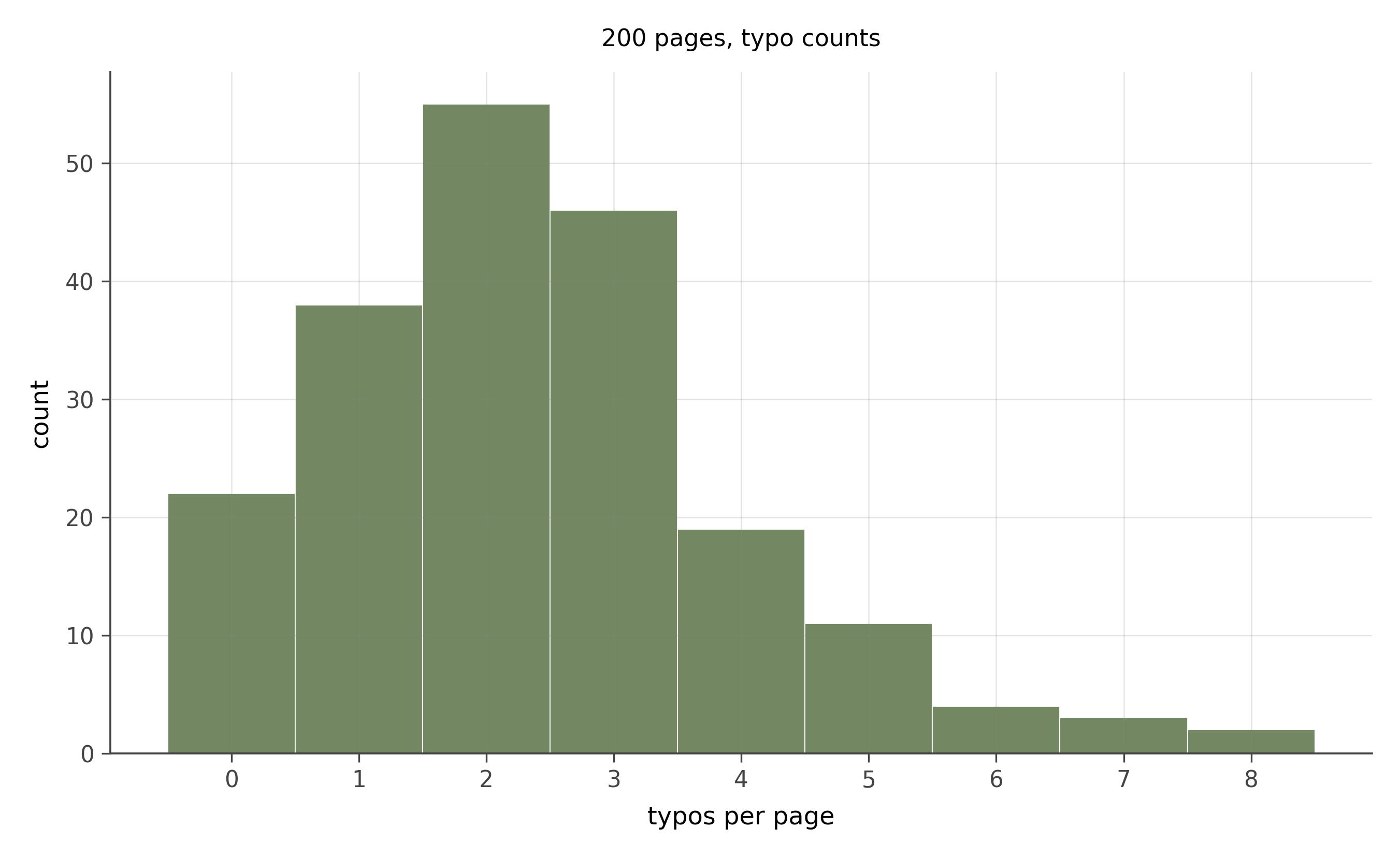
- What shape?
- What story produces it?
- Roughly what is the average number of typos per page?
Shape. Poisson. Right-skewed, supported on non-negative integers, peaked near 2 or 3.
Story. “Rare events in a fixed window.” Each typo is rare per word, the rate is approximately constant, and typos are roughly independent of each other. The count per page is then approximately Poisson.
Average. Visually the peak is near 2 or 3 and the tail extends out to 7 or 8. The mean is approximately 2.5. (Sanity check: for a Poisson, mean equals variance equals \lambda, so \sqrt{\lambda} \approx 1.6 should be the standard deviation. The histogram’s spread looks about right.)
14.2.2 Problem 4: Household incomes
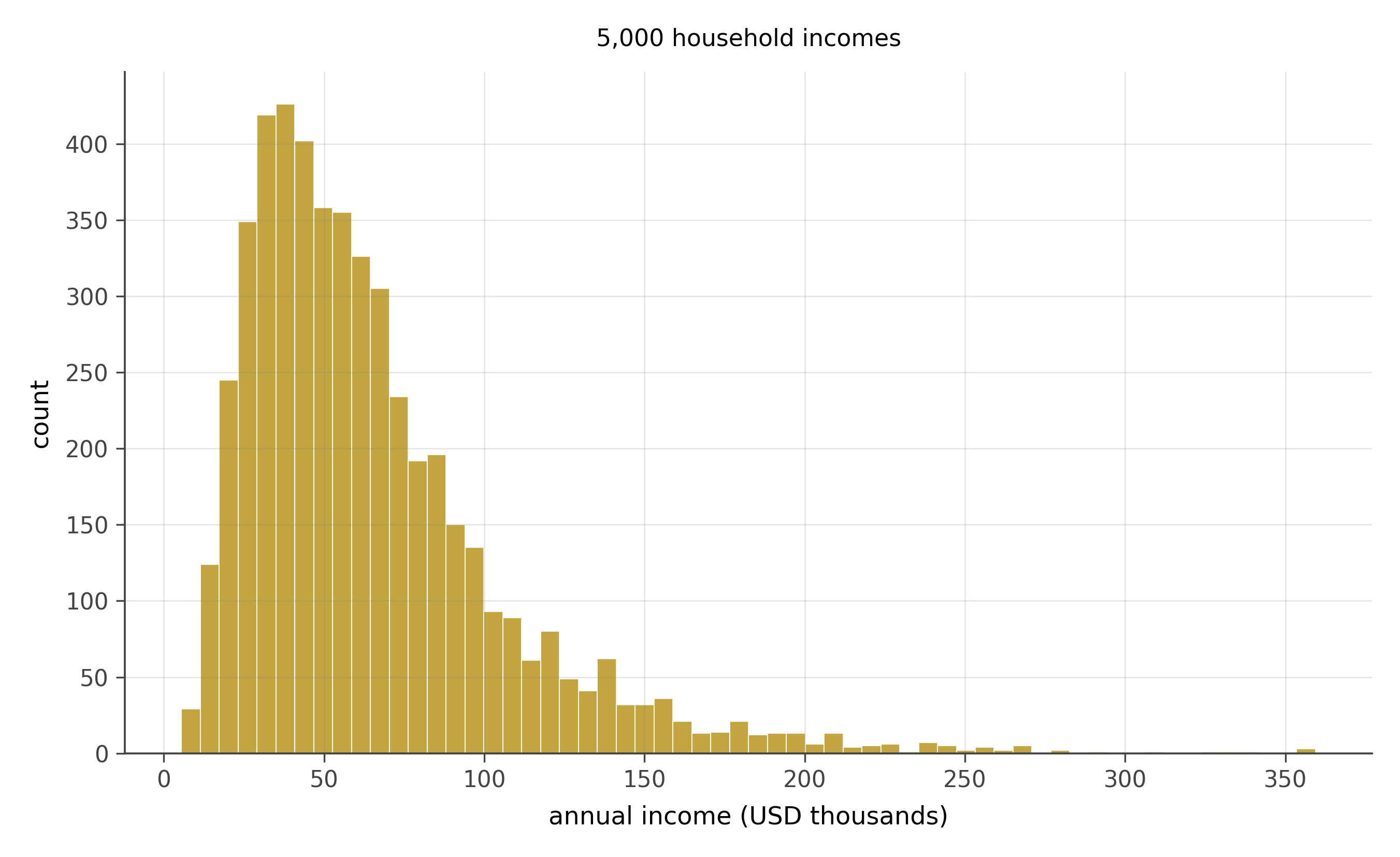
- What shape?
- What story?
- Should a journalist reporting this data quote the mean or the median?
- What happens if you take the log of the values and plot a new histogram?
Shape. Heavily right-skewed. Most of the mass clusters at moderate values; a long tail of high earners stretches to the right.
Story. “Multiplied small effects.” Income is the product of skill, education, opportunity, market conditions, and luck. Each multiplies the previous. The log of income is therefore approximately normal, which makes income itself approximately log-normal.
Mean or median. The median, almost always. The mean is dragged upward by a small fraction of very high earners. If a country’s median income is $50,000 and its mean is $80,000, the gap is the right tail. Reporting the mean exaggerates how a typical household lives.
Log transform. Take the log of each value. The new histogram becomes approximately normal: symmetric, single peak. This is the reflex move whenever you see right-skewed data. Log it and see if the result looks normal. Often it does.
14.2.3 Problem 5: Twenty coin flips, repeated
- What shape?
- What story?
- Where is the peak? Where do most values fall?
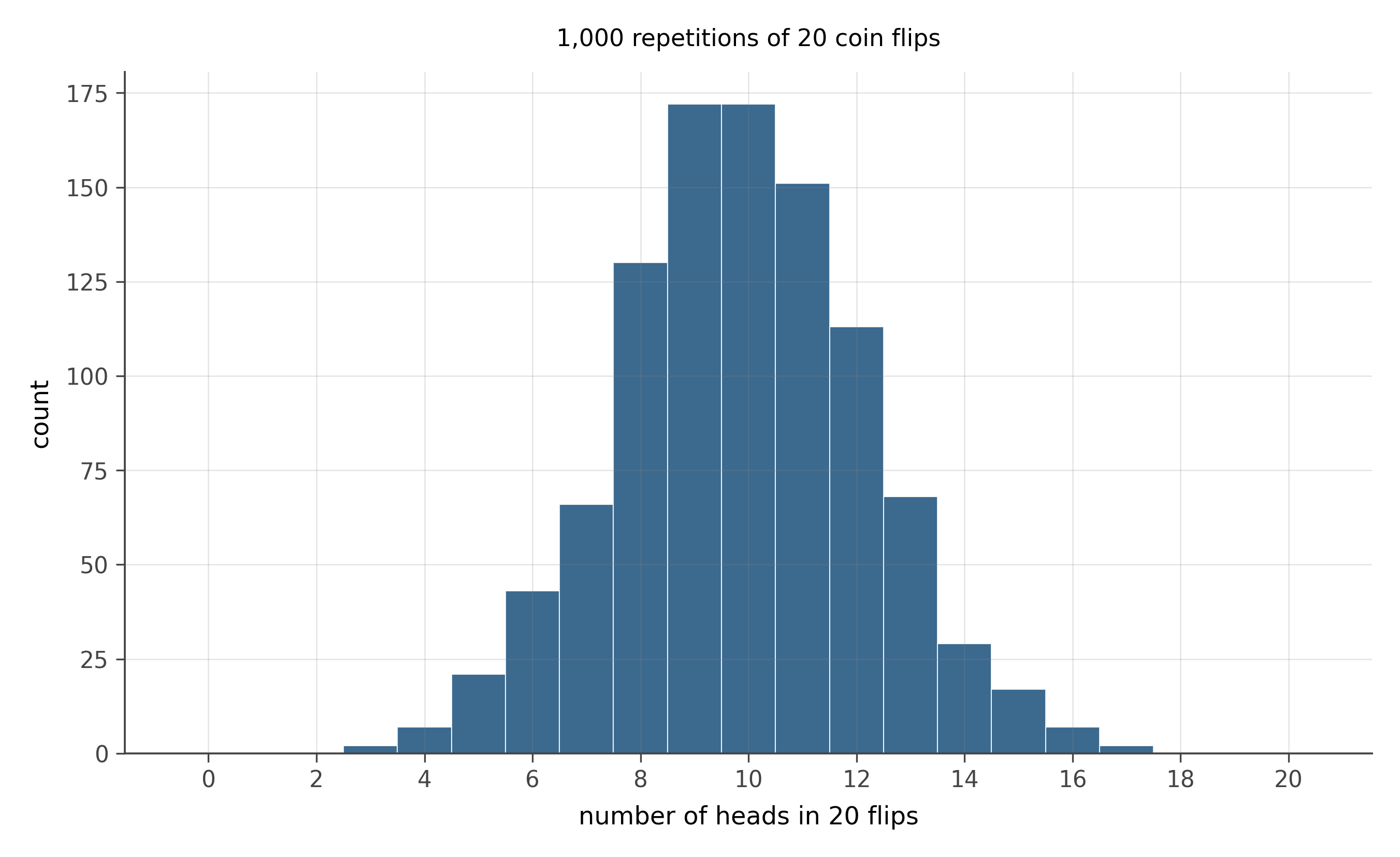
Shape. Binomial. Symmetric (because p = 0.5), peaked at 10, bell-shaped envelope.
Story. “Fixed number of trials, count the yeses.” With n = 20 trials and p = 0.5 probability of success per trial, the count of heads follows Binomial(20, 0.5).
Peak and spread. The peak is at np = 10. The standard deviation is \sqrt{np(1-p)} = \sqrt{5} \approx 2.24. By 68-95-99.7 (the binomial at this n is well-approximated by a normal), about 95% of values fall in 10 \pm 2(2.24) \approx [5.5, 14.5]. Almost all observations live between 5 and 15 heads.
14.2.4 Problem 6: Daily stock returns
- What shape?
- How does this differ from a normal?
- What is the practical implication for risk management?
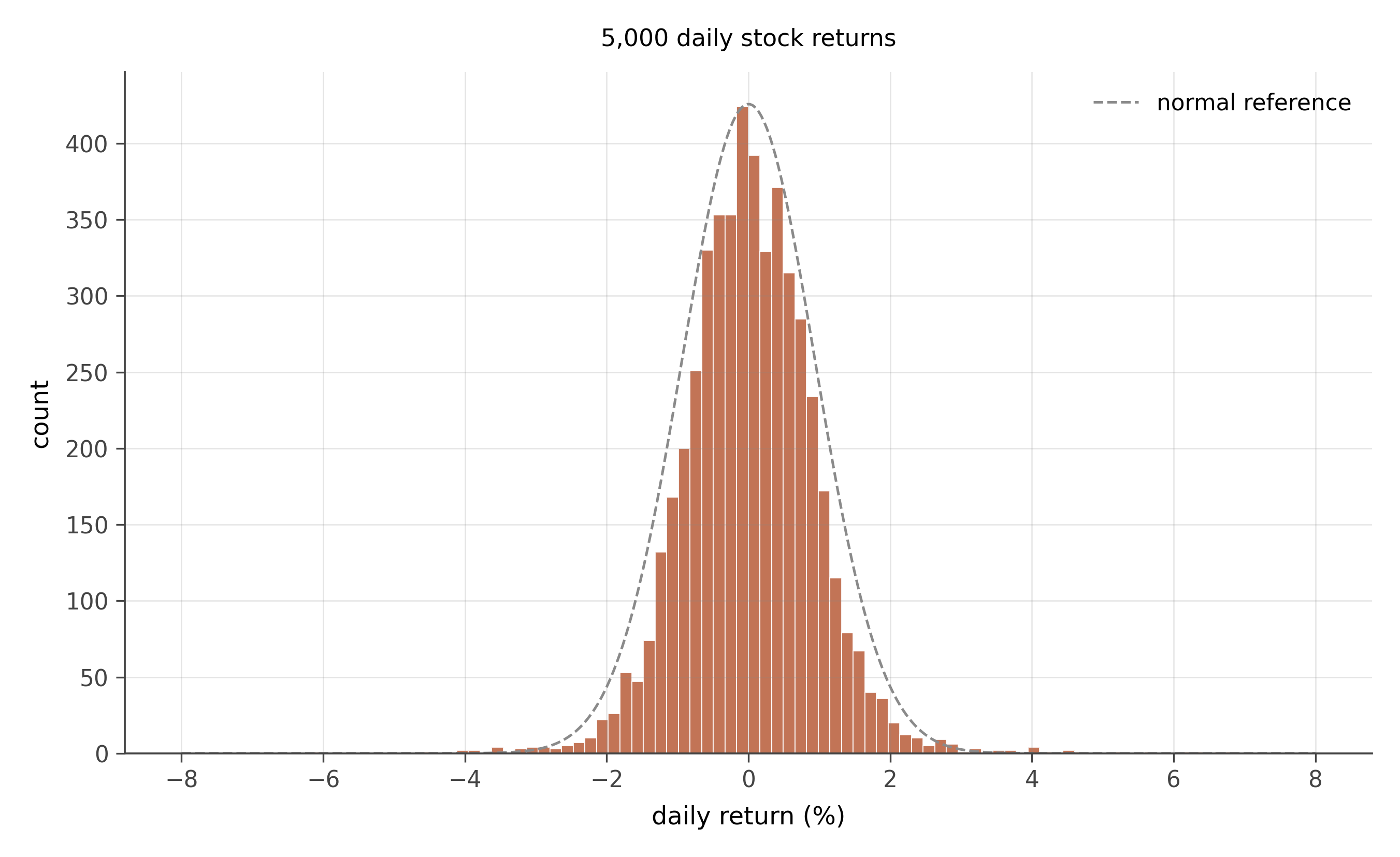
Shape. Roughly symmetric, peaked near zero, but with much heavier tails than a normal distribution. This is sometimes called “leptokurtic” or “fat-tailed.” Visually, the peak is taller than a normal of the same standard deviation, and the tails (events more than 3 standard deviations from zero) are noticeably more populated.
Difference from normal. Extreme returns (large positive or negative days) are more common than a normal would predict. A normal distribution with the same standard deviation would predict a 4-sigma daily return roughly once every 30,000 trading days. In real return data, 4-sigma days occur every few hundred days.
Risk management. Models that assume normal-shaped returns systematically underestimate the probability of large losses. The 2008 financial crisis is partly a story of risk models built on normality assumptions when the real distribution had much heavier tails. Modern risk modeling uses heavy-tailed distributions (Student’s t, generalized Pareto for the tails) to avoid this failure mode.
14.3 Stretch
14.3.1 Problem 7: Reaction times
- What shape?
- Why does the data take this shape?
- Should the experimenter report the mean or the median?
- What transformation makes this data easier to model?
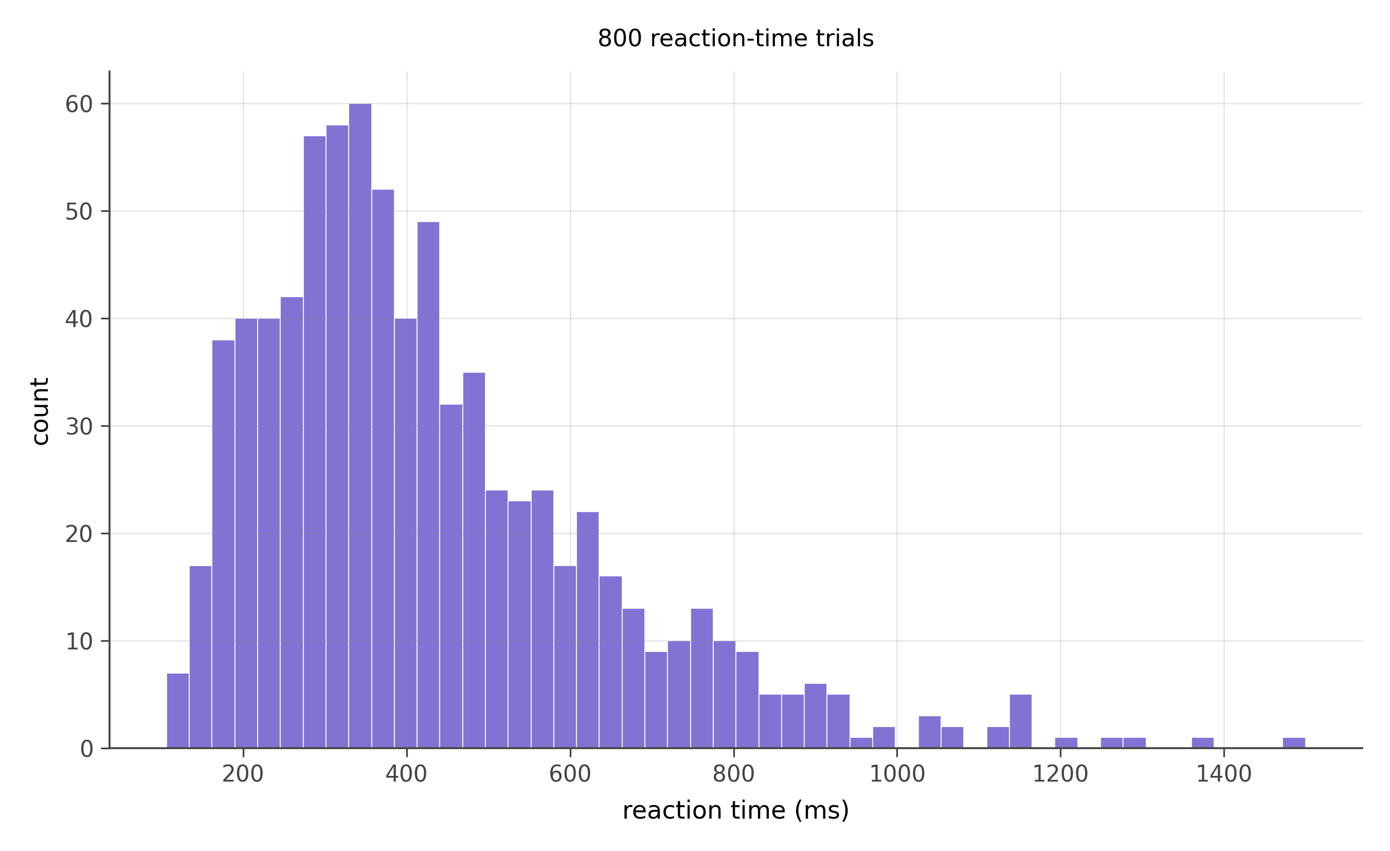
Shape. Right-skewed, with a peak around 350 ms and a long tail extending to 1500 ms or more.
Why. Reaction time is bounded below by neural transmission speed; you cannot react faster than your nervous system permits. It is unbounded above; you can react arbitrarily slowly when distracted. The lower bound builds a wall on the left; the unbounded right side opens a tail. Combined with the multiplicative nature of the stages of cognitive processing (signal detection × decision × motor response, each with its own variability), the result is approximately log-normal.
Mean or median. The median, for the same reason as income. A few very slow trials drag the mean upward and away from the typical response.
Transformation. Log-transform the reaction times. The result is approximately normal, which makes standard statistical methods (t-tests, regression) directly applicable. The cognitive psychology literature largely models reaction times on the log scale.
14.3.2 Problem 8: Bilateral trade volumes
- What shape on the linear scale?
- What shape on the log scale?
- What does this tell you about how trade economists actually fit regressions?
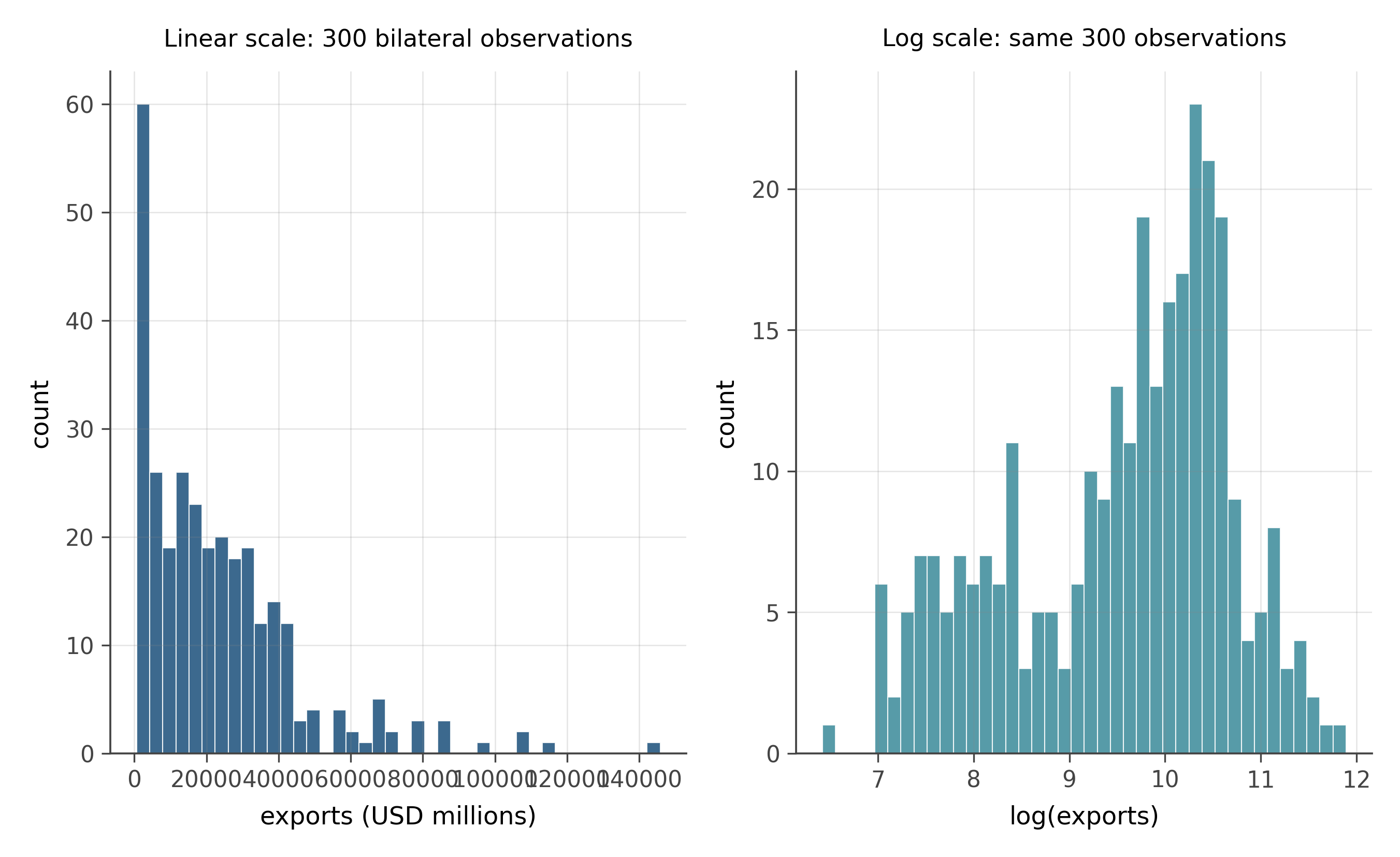
Linear scale. Heavily right-skewed. A small number of large bilateral relationships (USA-CHN, CHN-USA, USA-DEU) dominate the right tail; most pairs trade much less.
Log scale. Approximately symmetric and roughly bell-shaped. Log-trade is much closer to normal than trade itself, which is the log-normal pattern from problem 4 applied to a different domain.
Implication. Trade gravity equations are almost always written on the log scale: \log(\text{exports}) = \alpha + \beta_1 \log(\text{GDP}_{\text{exporter}}) + \beta_2 \log(\text{GDP}_{\text{importer}}) + \beta_3 \log(\text{distance}) + \cdots. Two reasons. First, log-trade is normal-shaped, which makes OLS work cleanly. Second, log-log regression coefficients are elasticities: a unit change in \log x is a percentage change in x, so the coefficient on \log(\text{GDP}) tells you the percent change in exports per percent change in GDP. That is the quantity trade economists want. When you read empirical trade papers in later chapters, almost every regression you see will have logged dependent and independent variables.
14.4 Real UK data
The two problems below use administrative data collected by UK government agencies. The Land Registry Price Paid Data records every residential property transaction in England and Wales registered with HM Land Registry; the 2024 extract contains approximately 93,000 transactions with price, property type, date, and location. The English Indices of Deprivation 2019 (IMD 2019), published by the Ministry of Housing, Communities and Local Government, measures deprivation across seven domains for every Lower Super Output Area in England — 32,844 small geographies of roughly 1,500 residents each.
14.4.1 Problem 9: UK house transaction prices
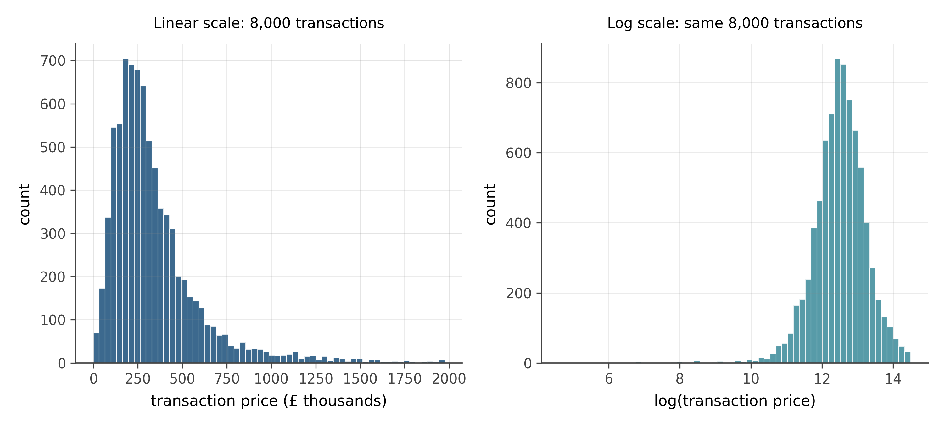
- What shape does the price distribution take on the linear scale?
- Which chapter-3 story explains why house prices take this shape?
- What happens to the distribution when you take logs? What does this tell you about the data-generating process?
- A newspaper headline quotes the mean house price in England as much higher than what most buyers actually pay. How does the shape of this distribution explain the discrepancy?
Shape on linear scale. Heavily right-skewed. The bulk of transactions cluster between £100,000 and £400,000, but a long tail extends toward £1,000,000 and beyond. This is one of the most common distributional shapes in economics.
Story. Multiplicative growth. A property’s price reflects a sequence of compounding influences: local wage levels, planning constraints, proximity to amenities, neighborhood reputation, historical appreciation, and market timing. Each factor multiplies rather than adds to the previous. The product of many small positive multiplicative factors converges to a log-normal distribution. The same story applies to income (workbook problem 4) and bilateral trade (problem 8).
Log transform. The log-scale histogram is approximately symmetric and bell-shaped, close to a normal distribution. This is the fingerprint of a log-normal: take logs and the result looks normal. The implication is that the data-generating process is fundamentally multiplicative.
Mean vs median. The long right tail drags the mean above the median. A small fraction of very expensive transactions (often in London and the South East) inflates the mean without describing a typical buyer’s experience. The median is the right summary for “what does a typical purchaser pay.” Policy discussions about housing affordability almost always use the median for this reason, though press reports sometimes quote the mean because it is larger and sounds more alarming.
14.4.2 Problem 10: English neighbourhood deprivation
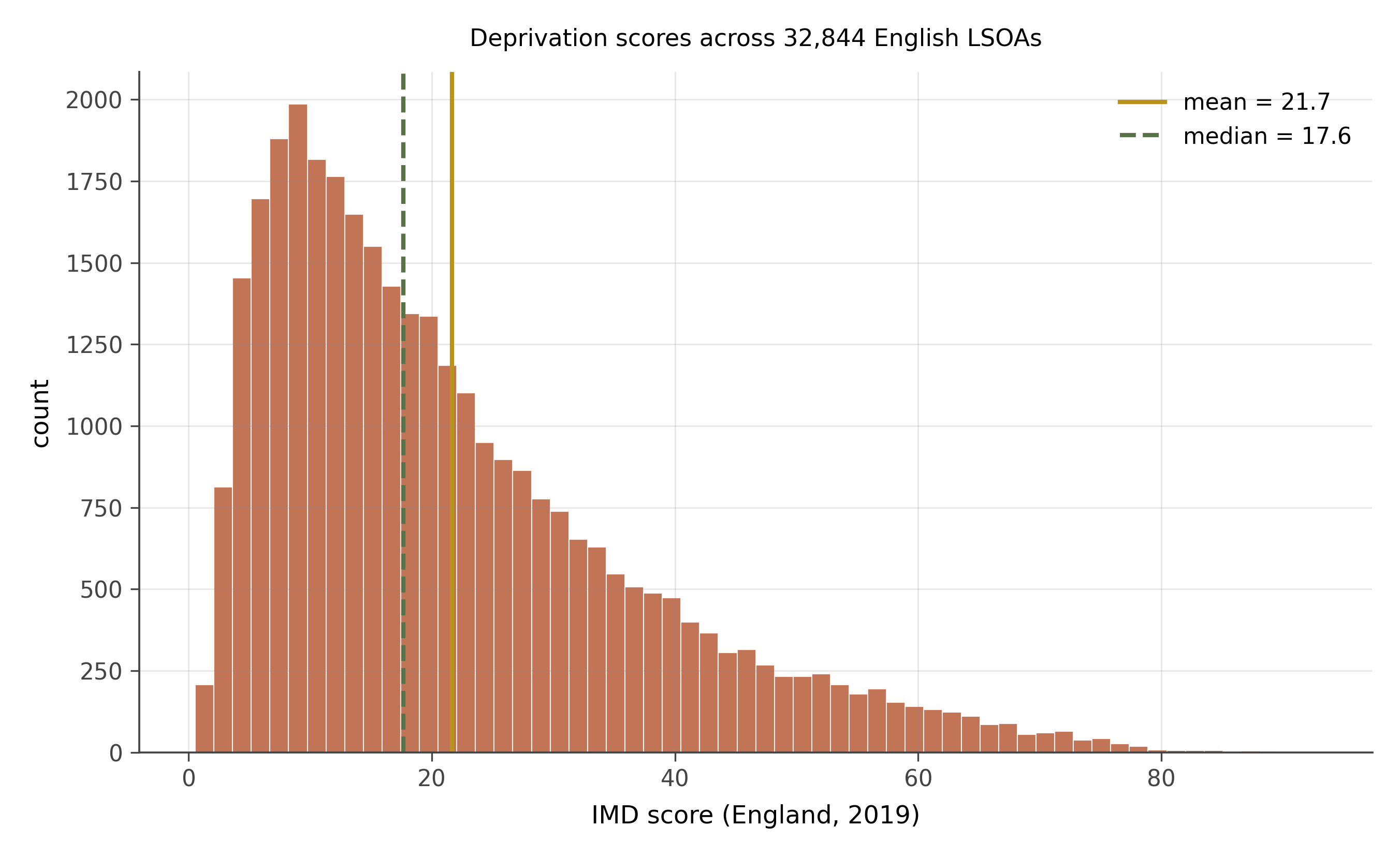
- Describe the shape of this distribution. Is it symmetric?
- The mean is noticeably higher than the median. What does this tell you about inequality in the data?
- A researcher claims that the “typical” English neighbourhood has a deprivation score of about 20. Is this a defensible claim? What would you need to know to assess it?
- If a government programme targets the most deprived 10% of areas, which statistical tool is most useful for identifying them: the mean, the median, or the rank/decile structure of the data?
Shape. Right-skewed. Most LSOAs have moderate scores (roughly 10 to 35), but a tail of very deprived areas stretches toward high scores above 50. The shape is smoother than income distributions but has the same basic skew: concentrated moderate deprivation with a smaller group of severely deprived areas.
Mean above median. In any right-skewed distribution, the mean is pulled upward by the long tail. Here, the areas of very concentrated deprivation (inner-city LSOAs in towns like Blackpool, Middlesbrough, and parts of London) drag the mean above where the bulk of the data sits. This is a direct measure of inequality: the greater the gap between mean and median, the more the distribution is dominated by extremes rather than the typical case.
Defending a claim about the “typical” neighbourhood. Whether a score of 20 is defensible depends on whether you use the mean or median. If the median is roughly 21–22 and the mean is higher, then “about 20” may be close to the median. The defensibility requires specifying which summary you are using and why. The median is more representative of the typical neighbourhood; the mean is more sensitive to the most deprived areas.
Targeting the worst-off 10%. The rank or decile structure is the right tool. The IMD data comes with pre-computed deciles and vigintiles (twentieths). Targeting “decile 1” areas directly selects the most deprived 10% without any ambiguity about mean versus median. This is a case where ranks are more decision-relevant than moments. Means and medians describe the centre of a distribution; ranks describe position within it.
14.5 What you practiced
By the time you finish this workbook, the shape-to-story matching should feel automatic. The pattern is:
- Look at the histogram.
- Symmetric or skewed? Heavy-tailed or light-tailed? Single peak or several?
- Match to one of the six chapter-3 stories.
- If right-skewed, take the log and replot. Often the log-version is normal-shaped, which unlocks every standard tool.
The next workbook (Reading regressions by inspection) extends this pattern to scatter plots and what they tell you about a regression before you fit one.