10 Underused visualizations
- Six chart types beyond the standard repertoire
- Slope graphs, Cleveland dot plots, hex bins, ridge plots, mosaics, alluvials
- Which question each one answers better than the conventional alternative
10.1 Beyond the standard repertoire
The standard chart repertoire in introductory courses is small: bars, lines, scatters, pies, histograms. Boxplots, if the instructor is feeling generous. Most students leave their first stats course with that as their entire vocabulary, and most working analysts add at most one or two more over the course of a career.
This is a poverty. The visualization literature has produced many chart types that answer specific questions better than anything in the standard repertoire. Knowing them is the difference between an analyst who reaches for a bar chart in every situation and one who reaches for the right tool. The chart types in this chapter are not exotic. They are well-understood, available in every plotting library, and disproportionately useful for the kinds of questions empirical research actually asks. They are simply not taught.
Six chart types follow. Each gets a section and a question. Read the figures first, the prose second.
10.2 The slope graph
Tufte’s slope graph is the answer to “how did things change between two points in time?” It is two columns of numbers connected by lines: the value of each unit at time A on the left, the value at time B on the right, a line connecting them. Lines that go up represent increases. Lines that go down represent decreases. The eye reads the slope of each line to compare changes across units.
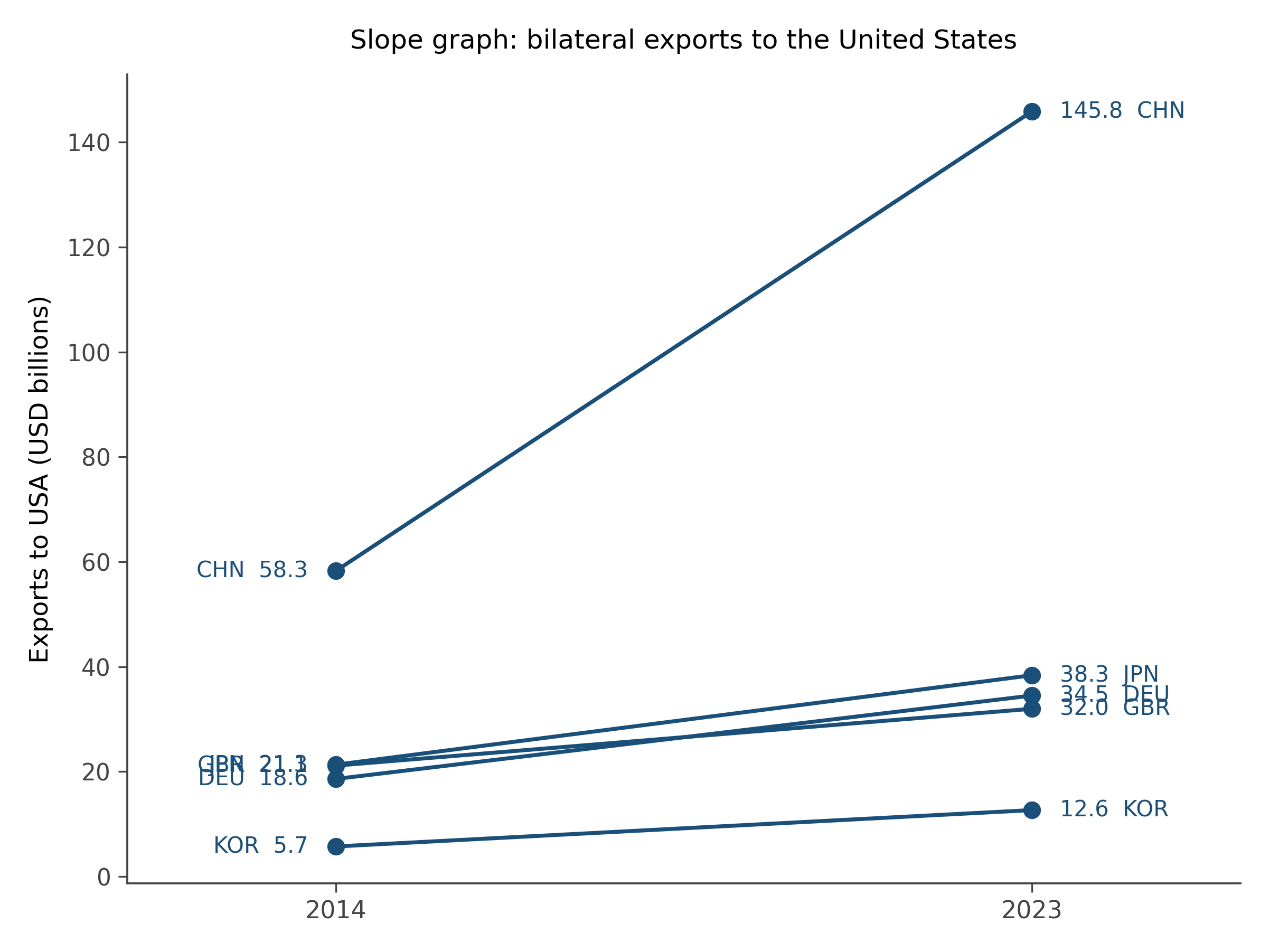
Why this works better than alternatives. A bar chart of differences answers the same question, but the slope graph also shows the levels at the start and end, which provides context. Two bar charts side by side answer the same question, but the eye has to do work to track which unit went where. The slope graph encodes change as the slope of a line; what the eye is asked to read is differences in slope, which is a much easier comparison than absolute angle.
When to reach for it. Two-point comparisons across many units. Survey results before and after an intervention. Pollutant levels at the beginning and end of a regulation period. Country-level outcomes across two policy regimes. The slope graph is at its best with somewhere between five and thirty units. Fewer is overkill; more becomes spaghetti.
10.3 The Cleveland dot plot
A Cleveland dot plot is a bar chart with the bars replaced by single dots. Each dot sits at the value, with a thin guideline back to a reference (often zero, sometimes the median). That is the entire chart.
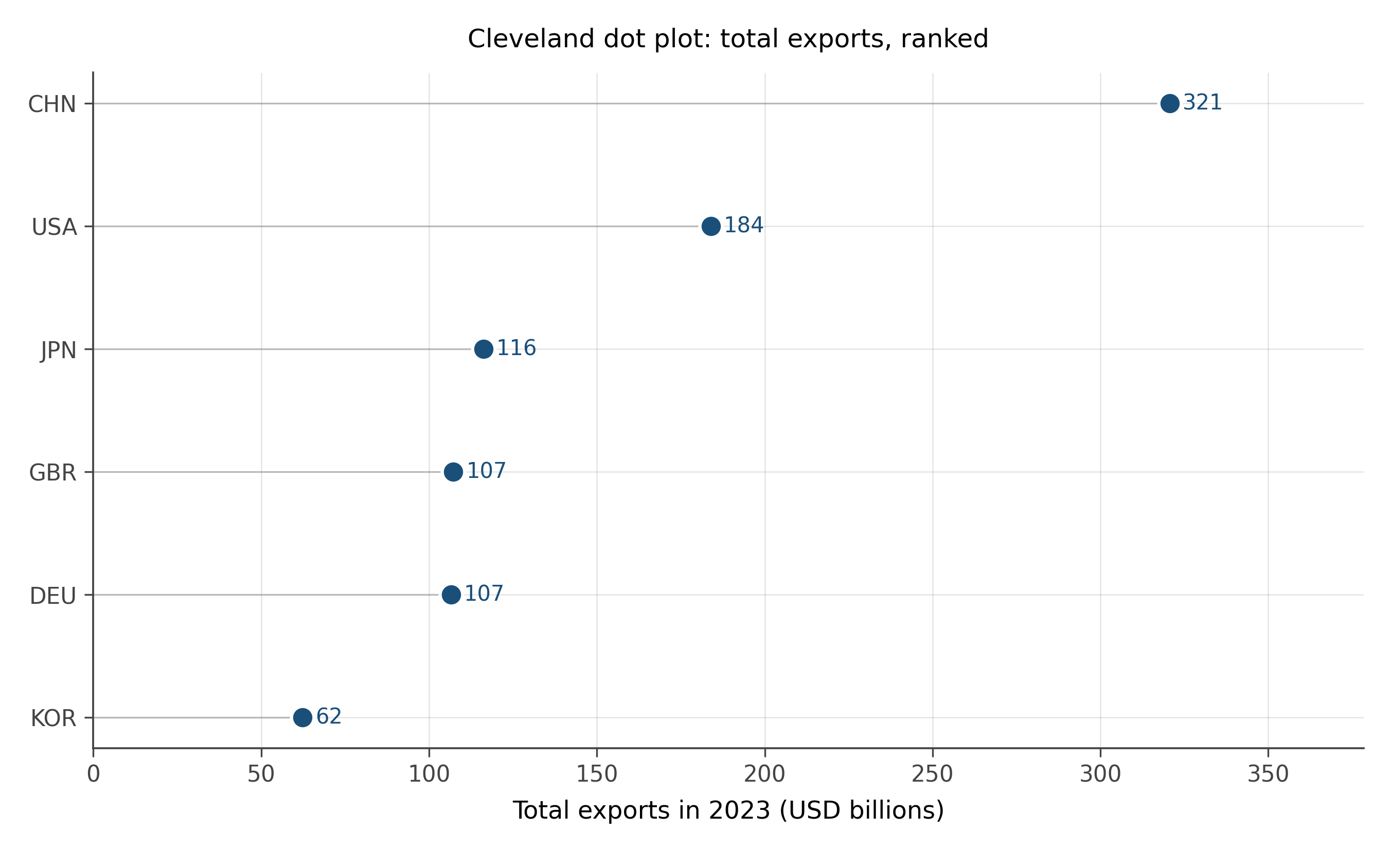
Why this is better than alternatives. Bar charts use ink to encode the same value twice: once as the position of the bar’s top, and once as the bar’s length. The eye reads position more accurately than length (per the perceptual hierarchy in chapter 4), so the body of the bar is decoration, not information. Dot plots strip the decoration. The result is more readable, especially when the number of categories is large.
The Cleveland dot plot is also better when the data does not start at zero, where bar charts become misleading (chapter 6). Dots can sit anywhere on the axis without implying a magnitude from the visual length of a bar. Stock prices, temperature anomalies, log-transformed values: all comfortable in dot plots, awkward in bars.
When to reach for it. Ranked comparison across many categories, especially when zero is not a meaningful reference. Country rankings, journal impact factors, expression levels across genes, performance benchmarks across teams.
10.4 The hex bin
A scatter plot stops working when there are too many points. With a thousand points, you can see structure. With a million, the points pile on top of each other and you see a black blob. The hex bin solves this.
A hex bin chart divides the plotting area into hexagonal cells and counts the number of points falling into each cell. Each cell is then colored by its count. Dense regions appear dark; sparse regions appear pale. The result is a heatmap of point density that reveals structure invisible in the underlying scatter.
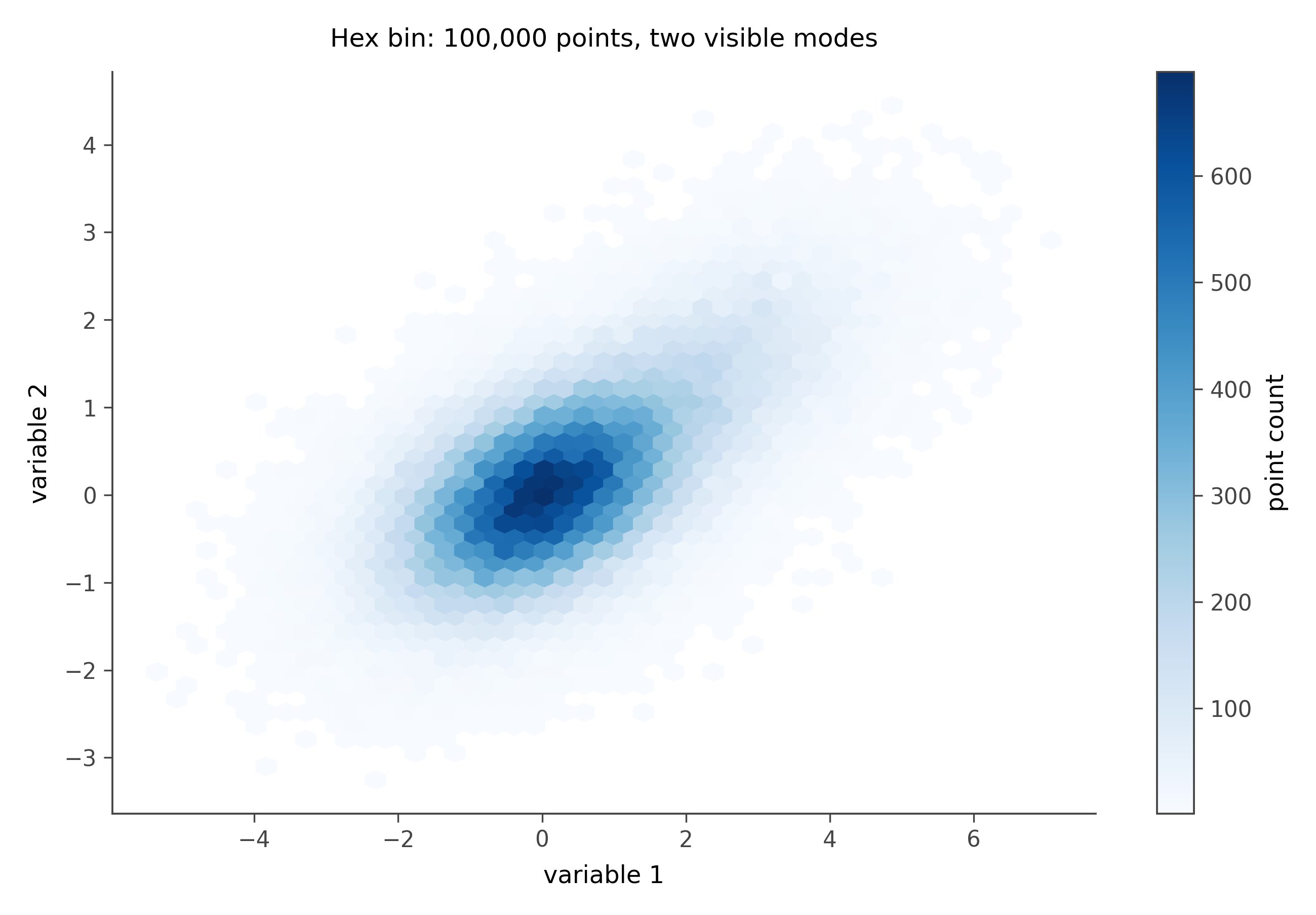
Why this works better than alternatives. With many points, a regular scatter is unreadable. A 2D histogram with rectangular bins is a step up but suffers from the rectangular grid showing through visually. Hexagons are nearly circular, which means they bin similarly in all directions, and they tile the plane without leaving gaps. The aesthetic result is smoother than rectangular bins and more accurate than a smoothed density plot for finding precise modes.
When to reach for it. Any scatter plot with more than about 5,000 points. Astronomy data, genomic data, large survey or transactional data, log files. If the underlying scatter would be a black blob, the hex bin is your friend.
10.5 The ridge plot
A ridge plot, sometimes called a joy plot, is a stacked sequence of small density plots, one per category, arranged vertically with each density slightly overlapping the one below. The result looks a bit like a topographic map of distributions.
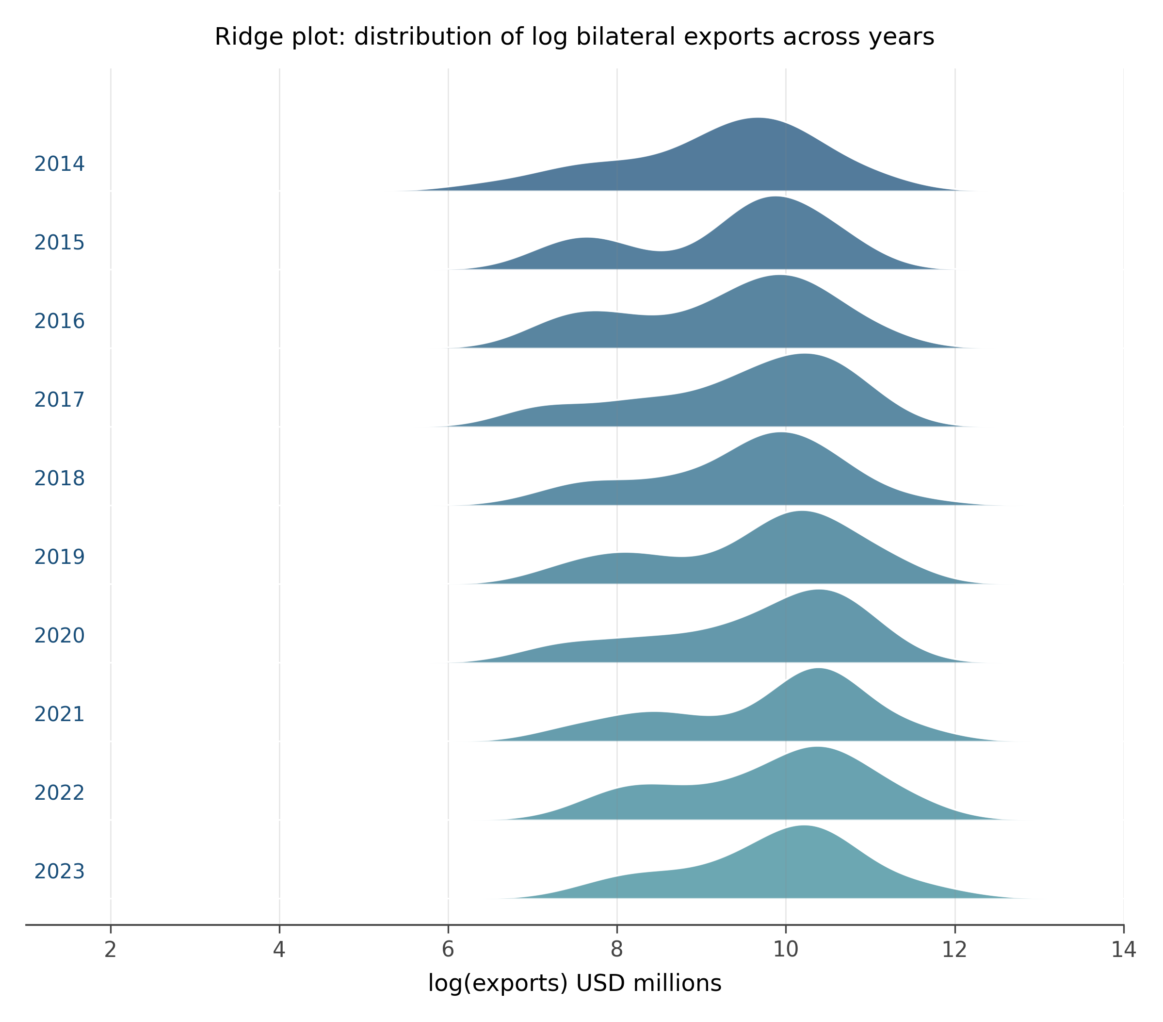
Why this works better than alternatives. To compare the distribution of a quantity across many categories (years, countries, conditions), the alternatives are: many small histograms (small multiples), violin plots side by side, or a single histogram colored by category (which becomes mush). The ridge plot is the most space-efficient of these for showing many distributions at once. The eye reads the shapes top to bottom and immediately spots which categories have unusual distributions.
When to reach for it. Comparing the shape of a distribution across five to fifty categories. Time-evolution of a distribution. Distribution of one variable across many groups. The ridge plot is what you want when the comparison is shape-vs-shape, not summary-statistic-vs-summary-statistic.
10.6 The mosaic plot
A mosaic plot is the visualization of a contingency table. The plot is a rectangle divided proportionally by one variable along one axis. Each resulting strip is then divided by another variable along the other axis. The areas of the resulting tiles are proportional to the joint counts.
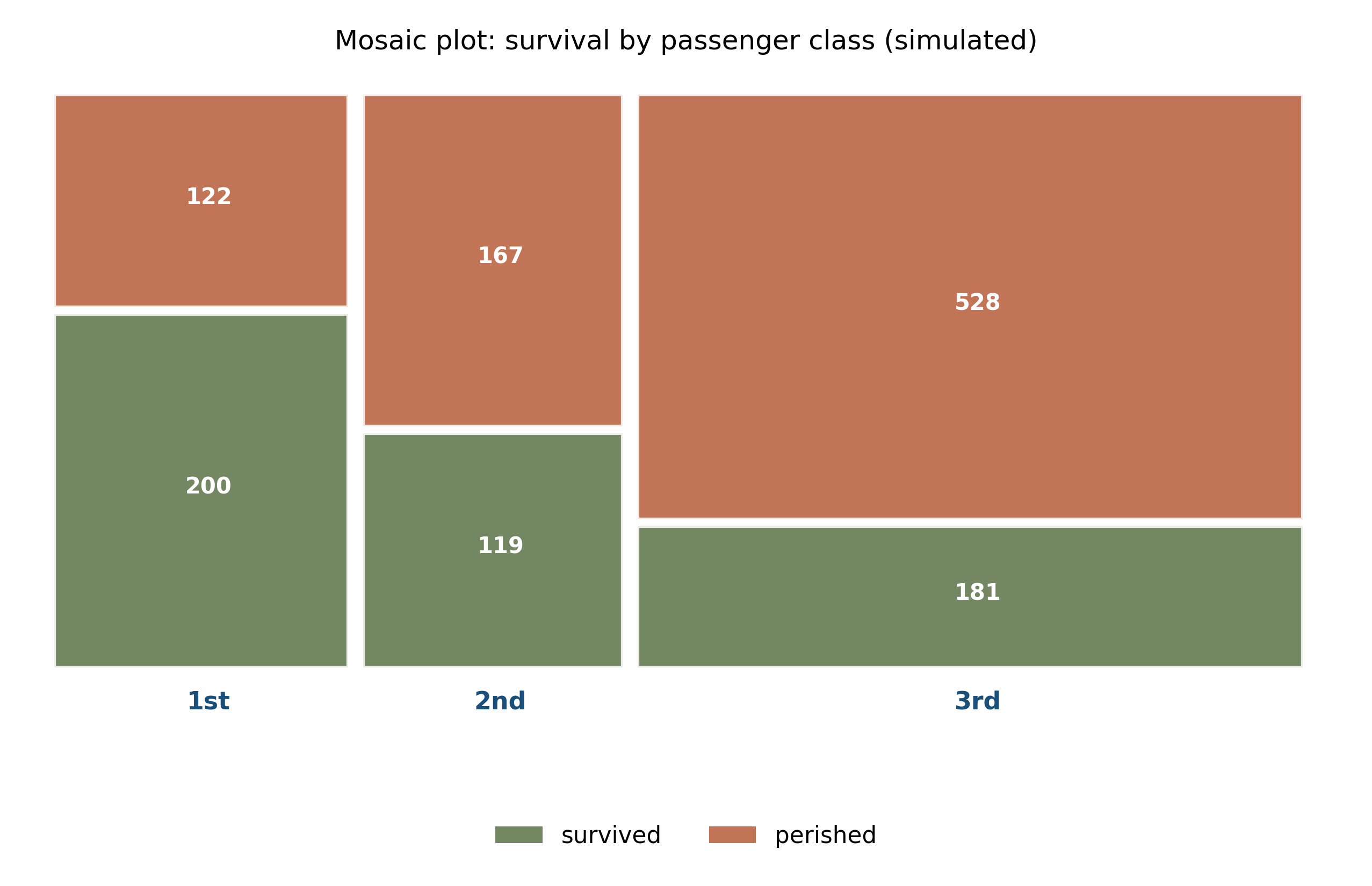
Why this works better than alternatives. A grouped bar chart of a contingency table answers questions about counts, but it does not show the marginal distribution of each variable, and it makes the joint distribution hard to read because the bars within a group are at different heights. The mosaic plot encodes everything at once: the marginal distribution along one axis, the conditional distribution within each level along the other, and the joint counts as areas. The eye spots which combinations are over- or under-represented relative to independence.
When to reach for it. Two or three categorical variables and you want to see association. Survival rates by class on a ship. Voting patterns by demographic and region. Confusion matrices in classification when you want to see joint structure beyond the diagonal.
10.7 The alluvial diagram
An alluvial diagram, in its directed-flow form often called a Sankey, shows how a population redistributes between categorical states. Stripes leave one set of categories on the left and arrive at another set on the right, with the width of each stripe proportional to the number of units making that transition.
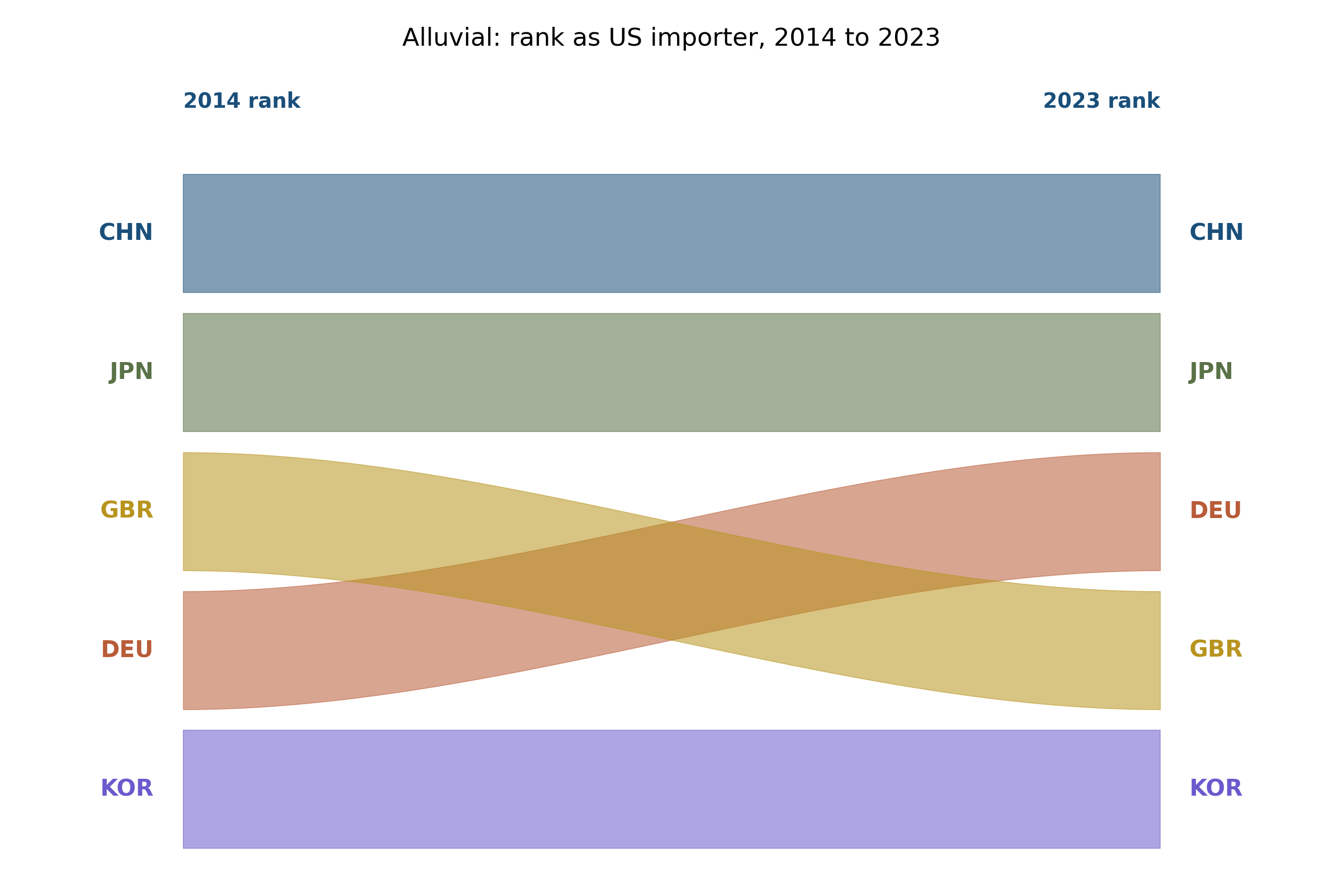
Why this works better than alternatives. Tracking flow between categories is hard with bars or lines. A grouped bar chart of “before” and “after” loses the connection between them. A Sankey or alluvial diagram makes the connection explicit: the visual width of each stripe is the number of units following that path.
When to reach for it. Categorical transitions over time or between conditions. Voter movement between elections. Customer-state movement (free → paid → churned). Trade partner reassignments. Employment-status changes. The alluvial is the right tool whenever the question is “where did they go?”
The standard chart repertoire teaches answers to a small set of questions. Each chart type in this chapter is the answer to a question the standard repertoire handles poorly. Knowing the right tool for the question is the difference between an analyst who fights their data and one who reads it.
For each scenario below, name the chart type from this chapter that fits best and explain why in one sentence:
- GDP per capita for 30 countries in 1990 and 2020. Show which countries gained ground and which lost it.
- A million bilateral trade flows. Reveal the joint shape of GDP and distance.
- A survey with five Likert items broken down by twelve demographic groups. Show how response distributions differ across groups.
- Students moving between four academic majors over four years of college. Display the dominant trajectories.
- Voting patterns by income decile and education level. Show which combinations vote which way.
After answering, draw at least one of these in a tool of your choice. The hardest part of using non-standard charts is reaching for them; once you do, the implementation is rarely the bottleneck.
The hex bin specifically uses hexagons rather than squares or triangles. The reason is geometric: among regular polygons that tile the plane, the hexagon has the most sides, which makes each cell closer to a circle.
For a square grid, a point near the corner of a cell is much further from the cell center than a point near the middle of an edge. This produces visible artifacts: the eye sees the grid even when the underlying data has no gridded structure. Hexagons reduce the effect dramatically. The visual texture of a hex bin chart is closer to the underlying density than any rectangular alternative.
This is the same reason bee hives, soap bubbles, and basalt columns are hexagonal: it is the most efficient regular tiling. Nature picks hexagons when packing matters; we pick them for the same reason in visualization.
Three questions to articulate in your own words before moving on:
Pick one chart type from this chapter you had never made before. What question does it answer that the standard repertoire could not?
Bar charts are the default for almost every quantitative comparison. Name a situation where you have used a bar chart that would have been better as a Cleveland dot plot.
The chapter argued that “the right tool for the question” is the design move. Where do you think your own default chart vocabulary is too small?
The visualization literature has produced many more chart types than the six in this chapter. Some that are gaining traction in modern empirical work:
- Parallel coordinates for high-dimensional data, showing many variables at once with one line per observation
- Heatmap matrices with hierarchical clustering for genomics and exploratory matrix data
- Network and graph layouts for relational data (which the trade panel of this book is, when treated as a directed graph)
- Calendar heatmaps for time-of-day, day-of-week patterns
The next chapter (visualizing uncertainty) covers a separate frontier: chart types that show not just the estimate but the uncertainty around it. Most of those are also underused outside of statistical specialty fields, even though they are exactly what the credibility revolution in empirical research is asking for.
10.8 Practice problems
Take any spreadsheet of two-time-point data you have access to. Render it as a slope graph. Count the number of lines that go up versus down. What story does the slope graph tell that you could not have read from the means alone?
The Cleveland dot plot uses position rather than length to encode magnitude. Design a dot plot for the data in the trade slice (USA’s exports to its five partners in 2023). Then redesign it for export change between 2014 and 2023. What changes between the two charts?
Pick a dataset with more than 10,000 rows and two continuous variables (any source: a research dataset, a public CSV, a log file). Make a regular scatter plot. Then make a hex-bin version. Compare what each chart reveals.
Find a contingency table in a recent paper or news article. Sketch it as a mosaic plot. What relationship between the variables becomes visible in the mosaic that was hidden in the table of numbers?
Construct an alluvial diagram for a categorical transition you actually care about (your students’ major changes, your team’s role transitions, partner shifts in a relationship dataset). The exercise is partly about whether the data lets you build it cleanly.
Looking ahead
Chapter 8: Visualizing uncertainty. Six new chart types in your hands. The next chapter turns to a separate frontier: how to show uncertainty as a first-class part of the visual story rather than as decoration on top of a point estimate. Continue →