When the model or the measurement changes

A model’s usefulness has a date

A forecasting procedure can be appropriate for one period and unreliable later. The underlying economic relation can change, the measurement instrument can change, or the decision can change. These are different reasons to revisit the procedure.

An expanding window uses a fixed starting date and accumulates observations. If a stable model is correct, more observations can improve estimation precision. If older observations describe a different regime, that same accumulation can anchor estimates to an obsolete relation. A rolling window discards older information, allowing faster adaptation at the cost of fewer observations and greater estimation variation.

Neither window is universally preferable. Their comparison concerns the tradeoff between sampling precision and relevance of past data. That tradeoff depends on the rate and form of change, the available sample, the model, and the decision loss.

Record an intended review schedule and an evidence-based retirement rule before deployment. Examples include an unrecoverable target-definition change, repeated forecast failures, sustained benchmark underperformance of economically meaningful size, or an identified input becoming unavailable. A model should not survive only because its original report was persuasive.

Write a break into the mechanism

The controlled experiment uses

$$Y_t=\phi_tY_{t-1}+\varepsilon_t, \qquad \phi_t=\begin{cases}0.8,&t<300,\\-0.4,&t\ge300.\end{cases}$$

The first regime has positive persistence; the second has alternating, quickly decaying dependence. The change is known to the experiment’s designer. The forecasting procedures do not receive the generating coefficients; they fit their declared windows at each origin.

In an empirical application, a break date may be uncertain. Selecting a date after inspecting the entire sample adds selection uncertainty and changes the inferential question. A historical break analysis and a sequential detector answer different questions: the former can use later observations to locate past change, while the latter must decide when change has become detectable.

This lecture does not treat a retrospective chosen date as a real-time detection result. It asks a narrower controlled question: how do two already specified estimation procedures behave after a change in the generating dynamics?

Bias and variance in a moving environment

In a stable AR process, a long window contains many relevant transitions. After a break, an expanding estimator mixes transitions generated by two different coefficients. Its fitted coefficient can converge toward a weighted compromise over the observation mix rather than the current regime’s coefficient.

A rolling estimator eventually contains only current-regime transitions, provided its window is shorter than the elapsed time since the break. Immediately after the break, however, it also contains old observations. The shorter window can react faster while remaining noisy. It may overreact to a run of unusual innovations even when no regime has changed.

The forecast consequences depend on the current level. A coefficient error multiplied by a large current deviation can create a large prediction error. A small coefficient change can matter economically when the action has asymmetric costs. Report loss in the action’s relevant units rather than treating coefficient stability as the only criterion.

Compare the same post-change targets

The source compares an expanding AR(1) and an AR(1) fitted on the most recent 80 observations. Both refit each period and forecast the same subsequent targets. Evaluation begins after 330 observations, so the design gives the procedures an initial post-break adaptation period. It does not measure their performance on the first surprise at the break itself.

That choice must be disclosed. A decision maker concerned with immediate disruption would also examine the transition targets and the first detection delay. A decision maker concerned with ongoing operation after the disruption could reasonably study the later window. The evaluation dates determine which question the reported losses answer.

For squared loss, retain paired differences

$$d_t=e_{\mathrm{rolling},t}^2-e_{\mathrm{expanding},t}^2.$$

Their mean describes the realized advantage of the rolling procedure on those targets. Dependence in $d_t$ complicates a standard error. The code also groups consecutive differences into non-overlapping blocks of ten and calculates the standard error of block means. This is a descriptive dependence-aware approximation at a short sample, not an automatic valid test under every break process. Lecture 4’s frameworks clarify why. The Giacomini–White framework supports normal or chi-squared inference for methods estimated on rolling windows of fixed length, but the expanding procedure here falls outside it. The Diebold–Mariano and West results assume a covariance-stationary loss differential, and a break that keeps moving the expanding estimate violates that assumption. The block and HAC standard errors therefore remain descriptive for this comparison.

Vary the block length and report sensitivity. Longer blocks can better retain dependence while providing fewer effective blocks. A narrow uncertainty estimate based on a single convenient block length should not decide a major model replacement by itself.

A measurement break can imitate an economic break

Suppose the economic state $S_t$ is stable but the indicator changes from $Y_t=S_t+\nu_t$ to $Y_t=a+bS_t+\nu_t$. A fitted autoregression can appear to change even though the latent economic dynamics have not. A new scale alters coefficients and forecast units; a new offset changes the mean; changing measurement noise changes apparent persistence.

Investigate metadata before changing the dynamics. Did geographic boundaries change? Did the provider redefine a sector? Did missing observations become zeros? Did the weighting scheme or seasonal adjustment change? An economic explanation and a measurement explanation can require very different repairs.

A documented conversion or crosswalk may restore comparability. A genuinely new economic regime may require a new model. If the old and new target cannot be reconciled, retire the historical series for the original task and define a new target. Extending a line through an incompatible definition does not create continuity.

Provider discontinuation is another operational issue. A model depending on a retired indicator cannot keep producing the same forecast without a substitute information source. An alternative measure needs its own validation; replacing a missing column with a similarly named series can change the economic construct.

Separate monitoring from repeated model selection

A monitoring system records performance, input availability, and model failures as outcomes arrive. A replacement process defines candidate repairs and evaluates them on an appropriate later boundary. If every surprising observation leads to a new model selected on all recent errors, apparent improvements can reflect repeated adaptation to noise.

Retain model versions and the dates their rules became active. Preserve the predictions actually issued. Recomputing historical predictions after every revision creates a revised backtest, not a record of deployment performance. The argument ledger should keep both the old decision and the new reasoning.

A practical review can produce three defensible actions: retain the current procedure, revise a specified component, or retire it and use a fallback. “Retain” is a substantive conclusion when the proposed repair lacks reliable benefit. “Retire” is appropriate when the target or information assumptions no longer support use.

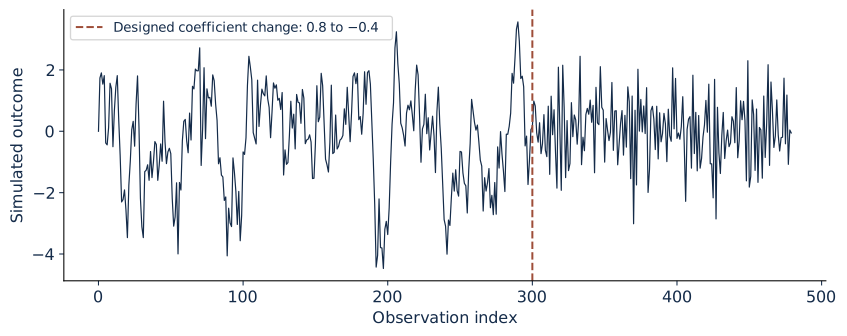
A designed persistence change, with its date known to the simulator. This figure is not a real-time break detector.

Execute, break, and repair

Run ch13. The shared realization estimates early persistence near 0.776 and late persistence near $-0.372$, reflecting the designed change. On the stated later targets, the rolling procedure has RMSE around 1.055 and the expanding procedure around 1.430. The paired loss difference favors the rolling procedure in this setting.

Now remove the break by keeping the generating coefficient at 0.8 throughout. Compare the same two window rules without changing the evaluation dates. The rolling procedure’s advantage need not remain. This is the essential negative control: a repair tailored to change can sacrifice precision when the process is stable.

Next move the break date and change its magnitude. Retain a small declared grid of sample sizes and window lengths. Record replication means and Monte Carlo uncertainty, including cases in which the ranking reverses. A course experiment should expose the conditions under which an argument fails, not only the example in which it succeeds.

Worked review decision

A deployed model’s mean monthly cost is 100 units over the review window, and a proposed repair has cost 97 on exactly the same targets. The numerical improvement is three units. If implementation costs are ten units per month, replacement is unattractive under that simple cost accounting even before statistical uncertainty is considered.

If the existing model’s required input disappears, the decision changes: its nominal historic accuracy does not restore feasibility. A less accurate but available fallback may become the defensible action. The ledger should identify feasibility and cost as separate dimensions.

For Project 3’s prototype, state which assumption the later release challenges and which repair addresses it. A revised pipeline should change only the components justified by evidence, preserving the comparison needed to assess the repair. Freeze that procedure before the continuation outcomes are examined.

Further reading

Forecasting: Principles and Practice on evaluation supplies the comparison framework. Provider-specific changes should be verified against the original dataset’s documentation rather than inferred from its graph alone.