Trends, unit roots, and misleading level regressions

Two rising series can have different mechanisms

A deterministic-trend model is $Y_t=a+bt+U_t$, where $U_t$ is stationary. A stochastic-trend model is $Y_t=Y_{t-1}+d+\varepsilon_t$. Their graphs can both rise. Their responses to a shock differ fundamentally.

In the first model, a disturbance to stationary $U_t$ eventually fades under stable dynamics and the series returns toward its deterministic path. In the second, a shock permanently changes the level of every future path. Subtracting a fitted line removes a deterministic trend under its assumptions; it does not eliminate the accumulated innovations of a random walk.

For the random walk, iteration gives $Y_{t+h}=Y_t+hd+\sum_{j=1}^h\varepsilon_{t+j}$. Its conditional forecast is $Y_t+hd$, and its known-parameter error variance is $h\sigma^2$. The forecast’s uncertainty grows with the horizon. A stable AR forecast’s variance instead approaches a finite limit.

If a series is stationary after one difference but not stationary in levels, we call it integrated of order one, $I(1)$, subject to the stated definition and regularity conditions. An $I(0)$ series has stationary behavior in the relevant sense. Integration order is a statement about a process; finite-sample tests provide evidence about that statement, not certainty.

Differencing removes a unit root and can create dependence

Define $\Delta Y_t=Y_t-Y_{t-1}=(1-L)Y_t$. A random walk with drift satisfies $\Delta Y_t=d+\varepsilon_t$. The accumulated stochastic trend disappears, leaving innovations and drift.

Differencing an already stationary white-noise series produces $\Delta Y_t=\varepsilon_t-\varepsilon_{t-1}$, an MA(1) with coefficient $-1$ under our sign convention. Its variance is $2\sigma^2$ and its lag-one correlation is $-1/2$. The root lies on the invertibility boundary. Over-differencing can therefore manufacture a distinctive negative correlation and increase noise.

An ARIMA$(p,d,q)$ specifies a stationary ARMA model for $(1-L)^dY_t$. Forecast the differenced series, then integrate predictions back to levels using the observed initial level. For $d=1$, a multi-step level forecast is the current level plus the sum of forecast differences. Its error variance requires covariances among those future difference errors; summing only their separate variances can be wrong.

Seasonal differencing $(1-L^{12})$ targets a seasonal unit root. It is a different operation from subtracting seasonal dummy effects or Fourier terms. Combining ordinary and seasonal differences requires a substantive reason and diagnostics; the appearance of a repeating seasonal pattern alone does not prove a seasonal unit root.

The Dickey–Fuller regression

Begin with $Y_t=c+\phi Y_{t-1}+\varepsilon_t$ and subtract $Y_{t-1}$:

$$\Delta Y_t=c+\delta Y_{t-1}+\varepsilon_t, \qquad \delta=\phi-1.$$

The unit-root null is $\delta=0$; the stable positive-persistence alternative has $\delta<0$. A DF statistic is the fitted coefficient divided by its estimated standard error. Under the unit-root null, its distribution is not the usual regression Student distribution. The regressor accumulates innovations, and the asymptotics involve functions of a stochastic path.

Deterministic terms matter. A regression without a constant, with a constant, and with a constant plus trend have different null distributions. Do not move a critical value across these specifications. Choose deterministic terms from the economic question and maintained model, then retain the correct reference distribution.

The augmented Dickey–Fuller regression adds lagged differences:

$$\Delta Y_t=c+bt+\delta Y_{t-1} +\sum_{j=1}^p\gamma_j\Delta Y_{t-j}+u_t.$$

The added terms address serial correlation under suitable conditions. Too few lags can leave dependence in $u_t$; too many can reduce power. Record the lag-selection rule and inspect residuals. Repeatedly trying deterministic terms and lags until a desired rejection appears changes the testing exercise.

A failure to reject does not establish that the process has a unit root. Near-unit stationary processes are hard to distinguish from unit-root processes in a short sample. A rejection can also be sensitive to a level break, trend break, or measurement change. Use the test with economic reasoning and later-target behavior.

The KPSS test of Kwiatkowski, Phillips, Schmidt, and Shin (1992) reverses the roles of the hypotheses. Its null is stationarity around the chosen deterministic terms, and its alternative is a unit root. It regresses $Y_t$ on those terms, accumulates the residuals into partial sums $S_t=\sum_{s\le t}\widehat u_s$, and compares $T^{-2}\sum_tS_t^2$ with an estimate of the residuals’ long-run variance. Its null distribution is also nonstandard, it depends on the deterministic terms, and the long-run variance requires a bandwidth choice. Reading the two tests together is informative. When the ADF test rejects and KPSS does not, the evidence favors stationarity; when KPSS rejects and the ADF test does not, it favors a unit root. When both reject or neither does, the sample has not settled the question, and a near-unit root, a break, or an unsuitable bandwidth are candidate explanations.

A finite-sample simulation of the test

The laboratory generates independent unit-root paths under a specified simple null: zero-drift Gaussian random walks initialized at zero. It fits a DF regression with an intercept, no trend, and no augmented lags. For sample sizes 80, 240, and 720, it repeats the experiment 2,000 times and records the proportion of statistics below $-2.86$.

That threshold is an approximate conventional large-sample 5% reference for the intercept specification. This simulation does not create a calibrated finite-sample critical value for every application. Its purpose is to reveal the sampling variation in a claimed rejection rate and the effect of sample size under this specific data-generating process.

Independent replications require independent draws, and the way a simulation is seeded can remove that independence without any visible error. The laboratory takes every path from one Park–Miller stream with a single documented seed and splits the stream into consecutive blocks of $n$ draws. An earlier version of this laboratory reseeded replication $i$ with $515+i$, and that scheme fails. The generator is multiplicative, so consecutive seeds produce first uniforms that differ by only $48271/(2^{31}-1)$. Over the 200 former replications, the first Box–Muller pair therefore always had a radius between 2.87 and 2.99, while its angle advanced by about 0.53 radians from one seed to the next. Across replications, the first two innovations each had a standard deviation of 2.07 instead of 1. The DF statistic with an intercept does not depend on the first draw of a path, but it does depend on the second, which had about four times its intended variance. Rejection rates computed that way therefore described a walk whose second step had the wrong distribution, drawn in replications that were not independent. Another base seed does not repair the scheme: seeds $2026+i$ over 2,000 replications give a first-draw standard deviation of 1.64. The code now records the standard deviation of the first draw across replications, which should be close to one, and the verification suite fails when it is not.

If $\widehat p$ is a Monte Carlo rejection proportion from $R$ independent replications, its approximate simulation standard error is

$$\operatorname{MCSE}=\sqrt{\frac{\widehat p(1-\widehat p)}R}.$$

With 2,000 replications, a proportion near 0.05 has an MCSE of about 0.005; with 200 replications it would be about 0.015, and differences of a few percentage points would be simulation noise. Increasing observations per replication and increasing replications address different uncertainties. The former changes the statistical experiment; the latter improves how accurately the simulation describes it.

The shared baseline produces rejection rates of 0.060, 0.0515, and 0.057 at $n=80$, 240, and 720, each with an MCSE of about 0.005. The reference script repeats the design with 200,000 replications from NumPy’s generator and obtains 0.054, 0.052, and 0.050, with MCSEs near 0.0005. Each course rate lies within 1.3 of its Monte Carlo standard errors of the corresponding reference rate. The small excess over 0.05 at 80 observations is a genuine finite-sample effect: $-2.86$ is an asymptotic critical value, and the 5% critical value for a sample of that length is slightly more negative. The differences among the course’s three rates are within simulation noise and say nothing about how size varies with sample length.

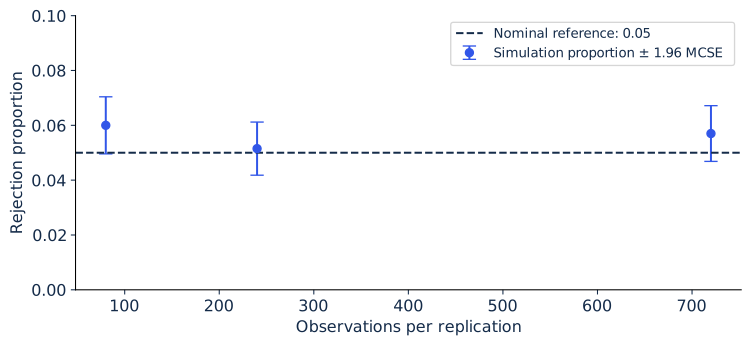
Dickey–Fuller size at the −2.86 reference: rejection proportions from 2,000 replications per sample size, drawn from one stream, with approximate 95% Monte Carlo error bars.

Why independent random walks can appear related

Suppose $X_t=X_{t-1}+v_t$ and $Y_t=Y_{t-1}+u_t$, with independent innovation sequences. Regressing $Y_t$ on a constant and $X_t$ in levels can generate misleading conventional significance. Each regressor carries a highly persistent random path. Usual stationary-regression laws do not justify the familiar standard-error calculation.

A single realization need not show the problem. The course’s baseline pair has a levels $R^2$ of about 0.0013 and a slope $t$ statistic of about 0.69. We retain that outcome, because the warning concerns the distribution of the procedure across many samples. The laboratory therefore repeats the experiment on 2,000 independent pairs of Gaussian walks for each sample size. The nominal 5% two-sided $t$ test of a zero slope in the levels regression rejects the true null in 74.8%, 84.4%, and 91.3% of replications at $n=80$, 240, and 720, with MCSEs of 1.0, 0.8, and 0.6 percentage points. After differencing, the same test rejects in 4.8%, 4.2%, and 5.0% of replications, close to its nominal size. The reference script’s 200,000 replications give 73.7%, 84.8%, and 91.2% in levels and 5.4%, 5.0%, and 5.0% in differences.

The false-rejection rate rises with the sample. Granger and Newbold (1974) documented the phenomenon by simulation, and Phillips (1986) explained it: in the levels regression the slope estimate converges to a random variable, while the conventional $t$ statistic diverges at rate $\sqrt n$. More data make the misleading inference more confident.

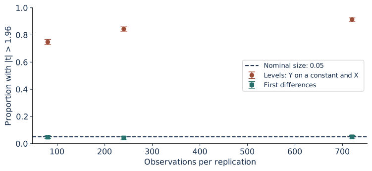
Proportion of 2,000 replications in which the nominal 5% $t$ test rejects a zero slope for independent Gaussian random walks, in levels and in first differences, with approximate 95% Monte Carlo error bars.

Differencing this example gives independent innovations, restoring the intended simple regression setting. But differencing every economic pair indiscriminately can discard a genuine long-run relation. Lecture 11 will construct two $I(1)$ series whose particular linear combination is stationary. Cointegration is the structured exception that must be investigated rather than assumed.

Execute, break, and repair

Run ch06 and inspect df_stat and unit_root_monte_carlo in the full source. Verify that the regression includes an intercept and that the reported statistic uses the lagged-level coefficient. Count the usable observations after differencing. The residual degrees of freedom are the number of usable rows minus the two fitted coefficients.

Deliberately compare the statistic with $-1.96$, the familiar normal threshold. Under this unit-root design, record how often that mistaken rule rejects. Restore the appropriate DF reference and compare. The repair changes the inferential rule; it does not change the fitted coefficient.

Next generate a deterministic trend plus a stable AR disturbance. Compare detrending and differencing using the correct target definition. Detrending estimates deviations from a deterministic path; differencing changes the series into period-to-period changes. Translate forecasts back into the original outcome units before comparing losses.

Finally add a known level break. Report how much the conclusions change when that break is represented explicitly. A unit-root decision should not be used to hide an obvious change in measurement or policy regime.

Worked problem and project audit

A random walk has drift 2, innovation variance 9, and current level 100. Its three-period forecast is 106 and its process-error variance is 27. A stable AR model with innovation variance 9 can also have a three-period variance near 27 when persistence is near one, but its long-horizon variance is finite if $|\phi|<1$. Short-horizon similarity does not establish identical long-run behavior.

For a stationary white-noise series with variance 9, the differenced series has variance 18 and lag-one covariance $-9$. Its lag-one correlation is $-0.5$. Seeing this pattern after differencing is a reason to examine whether the transformation was needed.

During the prototype exchange, audit the partner’s choice of levels, differences, and deterministic terms. Identify what observation would challenge that choice. A defensible audit can conclude that the available sample does not resolve the distinction and recommend robust short-horizon benchmarks. It should not convert an inconclusive test into a confident declaration.

Sources

Dickey and Fuller (1979) derive unit-root estimator distributions. Kwiatkowski, Phillips, Schmidt, and Shin (1992) test the stationarity null. Granger and Newbold (1974) and Phillips (1986) analyze spurious regressions. The practical ARIMA framework is discussed in Forecasting: Principles and Practice.