Estimating a latent state as observations arrive

Write the state and observation mechanisms separately

A scalar state-space model is

$$S_t=\phi S_{t-1}+\eta_t,\qquad Y_t=S_t+\nu_t,$$

where state innovations have variance $q$ and observation disturbances have variance $r$. In the elementary Gaussian version, both disturbance sequences are independent over time and independent of each other. The model separates an evolving economic quantity from a noisy observation of it.

The core exercise treats $\phi,q,r$ as given. Estimating all three adds identification, optimization, and initial-state questions. Those are useful extensions, but a working filter should first be understood with a transparent specified model. A smooth output alone cannot tell us whether its variance parameters are economically defensible.

If the state and observation share the same unit, $q$ and $r$ have squared units. A model with observation loading $\lambda$ would require consistent scaling: $Y_t=\lambda S_t+\nu_t$. The loading establishes how state units translate into indicator units. Without a normalization, latent scales can be arbitrary.

Predict the state before observing the new record

Let $m_{t-1}$ be the filtered mean of $S_{t-1}$ and $P_{t-1}$ its filtered variance, conditional on observations through $t-1$. The transition equation gives the prior prediction

$$a_t=\phi m_{t-1},\qquad V_t=\phi^2P_{t-1}+q.$$

The observation prediction is also $a_t$ because the loading is one and observation noise has mean zero. Its prediction-error variance is $V_t+r$. Define the observation innovation $v_t=Y_t-a_t$. This is an error in predicting the observed indicator; it is different from the unobserved state innovation $\eta_t$.

The new observation contains information about the state because $\operatorname{Cov}(S_t,Y_t\mid\mathcal I_{t-1})=V_t$. Under Gaussian conditioning, the state update is

$$K_t=\frac{V_t}{V_t+r},\qquad m_t=a_t+K_tv_t,\qquad P_t=(1-K_t)V_t.$$

The Kalman gain $K_t$ is dimensionless and lies between zero and one when $V_t\ge0$ and $r>0$. A noisy indicator gets a small weight; a precise indicator gets a large weight. The posterior mean is a weighted combination of the prior state estimate and the new observation.

The variance update follows from the same conditional-Gaussian formula: $P_t=V_t-V_t^2/(V_t+r)=V_tr/(V_t+r)$. It cannot exceed the prior variance. This is an analytic check that an implementation should preserve up to floating-point tolerance.

Check limiting cases

As $r\to\infty$, $K_t\to0$, and the observation contributes almost nothing. As $r\to0$ with positive prior variance, $K_t\to1$, the filtered state approaches the observed value, and posterior variance approaches zero. If $q$ increases, the prior becomes less precise and the new observation generally receives more weight.

If $\phi=0$, the prior state does not depend on the previous filtered state. If $q=0$, the state evolves deterministically from its initial uncertainty; repeated observations can progressively reduce uncertainty about that initial condition. Degenerate combinations require careful implementation to avoid division by zero or an unjustified stationary initialization.

For $|\phi|<1$, a stationary prior variance is $q/(1-\phi^2)$. The supplied code initializes the previous state mean at zero and variance at this stationary value, then applies the transition before the first observation. That convention implies the same stationary prior variance at the first observation. A diffuse prior or an economically informed initial state is a different specification.

Handle a missing observation by skipping its update

If $Y_t$ is missing, the state still evolves. Calculate $a_t$ and $V_t$, then set $m_t=a_t$ and $P_t=V_t$. There is no measurement update because no observation has arrived. Imputing $Y_t=0$ would instead treat zero as a real observation and could pull the state sharply toward it.

A run of missing observations increases uncertainty toward the transition model’s unconditional variance when the stable model applies. In an application, missingness may itself be informative. A measurement system that fails preferentially during extreme events violates the simple missing-at-random interpretation. The filter recursion can handle a missing input computationally while the underlying statistical assumptions remain questionable.

The data clock still applies. If the observation describes period $t$ but arrives later, update the model when it becomes available, using a properly specified delayed-observation system if necessary. Merely labeling it $t$ does not authorize an earlier update. The scalar exercise assumes observations arrive in their sequence at the stated dates.

Retrospective smoothing uses the future

After observing the entire sequence through $T$, a smoother estimates $S_t$ conditional on $\mathcal I_T$. Write its mean as $m_{t|T}$ and its variance as $P_{t|T}$; in this notation the filtered quantities $m_t$ and $P_t$ are $m_{t|t}$ and $P_{t|t}$. The scalar Rauch–Tung–Striebel recursion starts from $m_{T|T}=m_T$ and $P_{T|T}=P_T$ and moves backward:

$$J_t=\frac{P_t\phi}{V_{t+1}}, \qquad m_{t|T}=m_t+J_t(m_{t+1|T}-a_{t+1}),$$ $$P_{t|T}=P_t+J_t^2(P_{t+1|T}-V_{t+1}).$$

The backward correction uses what later observations reveal about earlier states. Under the specified Gaussian model, conditioning on more observations weakly reduces state uncertainty. The code checks that each smoothed variance $P_{t|T}$ is nonnegative and no larger than the corresponding filtered variance $P_t$. In the source, ms and Ps hold $m_{t|T}$ and $P_{t|T}$.

A smoother can improve historical state estimation while being unavailable for a real-time decision at that historical date. This is the model-based counterpart to Lecture 5’s centered average. Use filtered states to evaluate an earlier decision; use smoothed states to describe a retrospective reconstruction with its later information set stated.

The innovation likelihood and its limits

With specified Gaussian parameters, observation innovations give a log-likelihood contribution

$$\ell_t=-\frac12\left[\log(2\pi)+\log(V_t+r)+\frac{v_t^2}{V_t+r}\right].$$

Summing over observed dates supplies a likelihood objective for parameter estimation. Missing dates contribute no observation density while still changing the state prediction. Optimizing this objective requires admissible variance parameters, an initial-state convention, and checks for local solutions.

The standardized innovations $v_t/\sqrt{V_t+r}$ should have the assumed mean, variance, and dependence under a correctly specified model. Persistent correlation suggests missing state dynamics; unusual tails suggest a distributional mismatch; a variance shift can reflect a changing instrument or a changing state process. Estimating parameters does not eliminate the need to inspect these implications.

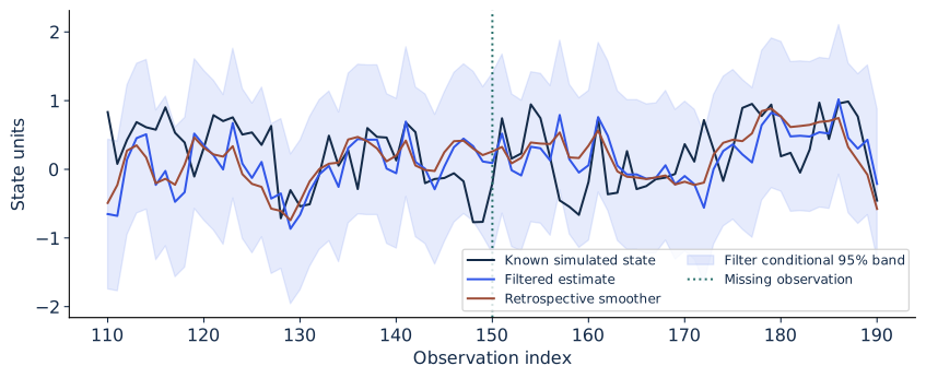
Known synthetic state, filter, and retrospective smoother. The shaded band uses the specified Gaussian filter variance; one observation is deliberately missing.

Execute and replicate independently

Run ch08. The generator uses $\phi=0.8$, $q=0.25$, and $r=1$, then deliberately removes one observation. The shared realization gives filter RMSE around 0.562 and smoother RMSE around 0.496 against the known simulated state. This comparison is possible because the simulation reveals its state; observed economic data generally do not.

The missing date’s filtered variance exceeds the preceding posterior variance. That result follows from skipping the update in this setting; the exact magnitude depends on parameters and prior uncertainty. Inspect the missing-value branch in every implementation and confirm it does not insert a zero observation.

Apply the future-mutation test by adding 10 to observations after index 180. The filter at 180 remains unchanged. The smoother at 180 changes materially because its later information changes. Freeze the parameter values during this comparison; otherwise a full-sample parameter refit can also change earlier filtered estimates.

Independently reproduce the first three updates by hand or in a short script before reading the implementation’s output. On the course’s audit day, protect time for this replication. A student who only reproduces the final graph has not demonstrated that the prediction and update steps are understood.

Worked update and project repair

Suppose the prior state mean is 10 and variance is 4, observation variance is 1, and the new indicator is 13. The gain is $4/(4+1)=0.8$, the posterior mean is $10+0.8(3)=12.4$, and posterior variance is $(1-0.8)4=0.8$. The observation moves the state toward 13 but does not eliminate uncertainty.

If observation variance instead equals 16, the gain is $4/20=0.2$, posterior mean is 10.6, and posterior variance is 3.2. The noisier observation contributes less information. If the observation is missing, the prior mean 10 and variance 4 remain the current estimate after the prediction step.

For Project 2, a measurement repair should state whether it changes the indicator, the state transition, the observation variance, or the admitted information. Do not replace a centered feature with a smoother and claim to have removed future dependence. An admissible repair must preserve the appropriate decision clock.

Sources

Kalman (1960) is the foundational filtering paper. Rauch, Tung, and Striebel (1965) derive the fixed-interval smoother. QuantEcon’s linear state-space lecture supplies a broader treatment.