A stable relation between moving levels

Integrated levels can share a stationary combination

Let $X_t$ be a random walk and let $Z_t$ be stationary. Define

$$Y_t=\beta X_t+Z_t.$$

Both $X$ and $Y$ can be $I(1)$, yet $Y_t-\beta X_t=Z_t$ is $I(0)$. The vector is cointegrated: a particular linear combination removes the shared stochastic trend. This is a restriction on joint behavior that is absent from the independent random walks in Lecture 6.

An economically motivated spread can arise between related prices, exchange-rate components, or quantities connected by a long-run accounting or adjustment relation. The economic reasoning proposes a candidate relation; the data and model assumptions determine whether it is credible. A high level-regression $R^2$ alone does not establish cointegration.

Units matter. If $Y$ and $X$ have different units, $\beta$ converts units so the spread is defined coherently. In log-price models, the coefficient may describe proportional long-run movement. A coefficient estimated on nominal values can change when currency units change even though the equivalent relationship remains intact.

Derive an error-correction model from a controlled mechanism

Suppose

$$X_t=X_{t-1}+v_t, \qquad Z_t=\rho Z_{t-1}+\eta_t, \qquad |\rho|<1,$$

and $Y_t=\beta X_t+Z_t$. Subtract lagged $Y$:

$$\Delta Y_t=\beta\Delta X_t+(\rho-1)Z_{t-1}+\eta_t.$$

Replace $Z_{t-1}$ by $Y_{t-1}-\beta X_{t-1}$:

$$\Delta Y_t=\alpha(Y_{t-1}-\beta X_{t-1}) +\beta\Delta X_t+\eta_t, \qquad\alpha=\rho-1.$$

This is an error-correction representation. A positive spread predicts a decline in $Y$ relative to the shared trend when $\alpha<0$. The lagged deviation supplies information lost by a regression containing only changes.

The derivation also supplies a stability restriction. Here $\rho=1+\alpha$, so $|1+\alpha|<1$, or $-2<\alpha<0$, makes the spread stable. A negative adjustment coefficient alone is insufficient: $\alpha=-3$ implies $\rho=-2$, an explosive alternating deviation. An adjustment coefficient between $-1$ and zero gives monotone mean reversion; between $-2$ and $-1$ gives oscillating mean reversion in this simple setting.

In a general multivariate system, several variables can adjust to the deviation. Then the relevant stability condition involves the combined adjustment and cointegrating vectors, not only one equation’s coefficient. Keep the scalar example’s restriction within the model from which it was derived.

The long-run and short-run coefficients need not match

The constructed mechanism makes the coefficient on $\Delta X_t$ equal to the long-run coefficient $\beta$. A more general single-equation ECM is

$$\Delta Y_t=c+\alpha(Y_{t-1}-a-\beta X_{t-1}) +\sum_j\gamma_j\Delta Y_{t-j} +\sum_j\delta_j\Delta X_{t-j}+u_t.$$

Its short-run response coefficients need not equal the long-run relation. Additional lags can represent delayed adjustment, while deterministic terms specify the equilibrium relation and drift. Define whether an intercept or trend belongs inside the cointegrating combination or outside it in the change equation; those choices impose different restrictions.

An equilibrium error is a model-defined deviation, not proof that market forces must eliminate it profitably. Transaction costs, structural changes, and unmodeled risk can affect both the relation and the interpretation. A stable statistical spread does not automatically create a tradable strategy after costs.

Estimate carefully and use the correct residual test

A basic two-step procedure estimates a long-run level relation and then uses its residual in an ECM. Under cointegration and suitable assumptions, the level slope has a distinctive convergence rate. Familiar stationary-regression standard errors are not automatically valid for every inferential claim in that first step.

Residual-based cointegration testing also requires a different reference distribution from an ordinary unit-root test on an observed series. The residual was constructed using estimated long-run coefficients. Applying an ordinary DF critical value directly to that estimated residual can overstate evidence for cointegration.

Deterministic terms, sample size, lag augmentation, and the number of variables affect the test specification. Use an implementation that documents the relevant cointegration test and retain its settings. The core laboratory deliberately avoids claiming a cointegration-test p-value from its plain residual regression. It constructs cointegration by design, then studies estimation and adjustment behavior.

For an applied case, examine whether each level plausibly has the required integration behavior and whether the proposed spread is stable. Investigate breaks in the economic relation and data definitions. Do not infer a stable equilibrium merely because a single test rejects in one conveniently selected window.

A vector error-correction representation

A VAR in levels can be rewritten

$$\Delta Y_t=\Pi Y_{t-1} +\sum_{j=1}^{p-1}\Gamma_j\Delta Y_{t-j}+u_t.$$

For rank $r$ with $0<r<m$, write $\Pi=\alpha\beta'$. Columns of $\beta$ describe $r$ cointegrating combinations; columns of $\alpha$ describe how variables adjust to them. The factorization has normalizations because $\alpha\beta'$ is unchanged by appropriate invertible transformations of those factors.

This connects multivariate dynamics to the common-trend restriction. Full-rank $\Pi$ corresponds to a stationary level system in the appropriate setting; zero rank removes the error-correction term. Determining rank and estimating a full Johansen system requires additional material. The core course stays with a transparent bivariate relation and uses the matrix form to explain what a system extension would add.

Forecast changes and return to levels

An ECM forecast combines the current equilibrium deviation, lagged changes, and admissible forecasts of future inputs. In the simple constructed model, if $\mathbb E[\Delta X_{t+1}\mid\mathcal I_t]=0$,

$$\widehat{\Delta Y}_{t+1|t}=\alpha\widehat Z_t, \qquad \widehat Y_{t+1|t}=Y_t+\alpha\widehat Z_t.$$

Using realized future $\Delta X$ supplies a conditional retrospective calculation, not an unconditional origin-time forecast. Forecast the input, specify a scenario, or model the system jointly. Uncertainty in the long-run relation and input forecast contributes to predictive uncertainty.

A forecast in changes must be evaluated in the correct target units. If the decision concerns the price level, reconstruct the level from the known current price. A model can predict changes modestly while still improving an economically important spread or level forecast; define the loss accordingly.

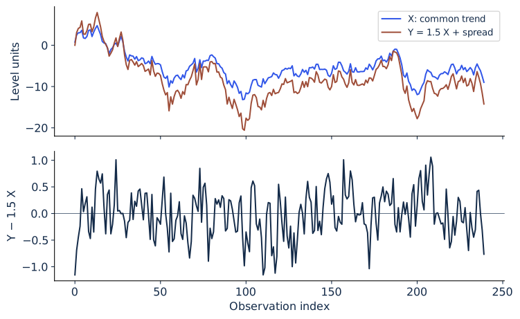
Two simulated integrated levels share a stationary spread by construction. This design supplies the truth; empirical cointegration requires investigation.

Execute and test the adjustment mechanism

Run ch11. The common trend is a simulated random walk; the true slope is 1.5; the spread follows an AR(1) with coefficient 0.5. Thus the generating adjustment coefficient is $-0.5$. The shared realization estimates the long-run slope near 1.503 and adjustment near $-0.506$.

Inspect the fitted spread, its variance, and its lag-one persistence. Compare the ECM’s residuals with those of a regression in changes that omits the equilibrium error. The latter discards an available predictive component in this constructed setting. Verify that the lagged spread is paired with the subsequent change, not with a change that precedes it.

Break the system by replacing the stationary spread with a second independent random walk. The resulting level relation no longer has the same constructed equilibrium. A finite sample may still look suggestive. Repeat the experiment and use the appropriate inferential framework before asserting a long-run relation. Repair the claim by narrowing it to the supported joint behavior or changing the model after documented evidence.

Worked problem and revision decision

Let the equilibrium relation be $Y=2X$, and suppose $Y_t=110$, $X_t=50$, and $\alpha=-0.25$. The deviation is 10. If the expected next change in $X$ is zero, the predicted change in $Y$ is $-2.5$ and the predicted level is 107.5. If expected $\Delta X$ is 3 and its short-run coefficient is 1.5, predicted change becomes $-2.5+4.5=2$, giving level 112.

The long-run coefficient 2 and short-run coefficient 1.5 answer different questions. A ledger that records only “the effect of X is 2” suppresses that distinction. Record the equilibrium definition, adjustment rule, input forecast, and the loss relevant to the decision.

Project 3 begins with a later data release. If the release challenges a claimed long-run relation, the response can be to revise the relation, retain a simpler procedure, or retire the model. Evidence that a historical spread was stable does not guarantee its future stability.

Sources

Engle and Granger (1987) develop cointegration and error-correction representations. Statsmodels’ VECM documentation describes the matrix form and deterministic-term conventions.