Lecture 2 of 15
Persistence, recursion, and aggregation
How does a shock persist, and what changes when observations are aggregated?
Prerequisites: Lecture 1, geometric series, covariance, and conditional expectation.
Unzip the bundle, open its code folder, and run ch02 in Python, R, or Julia; the entry point loads the course file and data beside it.
A model for a persistent economic level
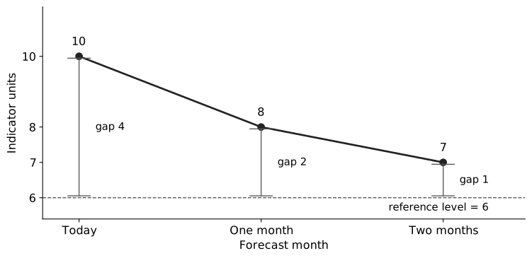
Suppose a monthly economic indicator is 10 today. We need a forecast for the next two months. Our model adds 3 each month and carries forward half the previous value. With no new shock, next month’s value is . One month later it is .
Why does the forecast move down? A value of 6 reproduces itself: . Today the indicator is 4 units above that level. One step leaves half the gap; two steps leave a quarter. We can therefore calculate the same two-month forecast as . These are invented numbers for a hand calculation; they are not estimates for the Texas electricity case.
Now write the rule as
The model is an autoregression of order one, abbreviated AR(1). Here and . The coefficient describes how much of a deviation survives one period. The intercept is the increment in the recursion; the reference level is when . The innovation is what the previous information could not predict. Its zero conditional mean lets the calculations above serve as forecasts even though future shocks will usually be nonzero.
The conditional-mean restriction rules out predictable innovations. Serially uncorrelated errors alone do not imply independence, Gaussianity, or this restriction. The second moment displayed above is unconditional: it averages across histories. It does not require the risk faced at each history to be the same. We will state the stronger condition when we calculate a conditional forecast variance. Treat and as known until the section on estimation uncertainty.
Here contains the observations and innovations through ; these information sets grow as records arrive. The known recursion lets us recover an observed innovation as . All innovations have finite second moments. These conditions make the conditioning steps below meaningful.
Lecture 1’s conditional-expectation proof explains why averaging the unknown future given today’s information minimizes squared forecast loss. Here we apply that result to a specific recursion.
If is in MWh, and are in MWh and is dimensionless. The interval represented by one time step matters. A monthly persistence coefficient cannot be substituted directly into a quarterly recursion.
Solve the difference equation
Substitute the recursion repeatedly:
To see the pattern, the first substitution gives . One more substitution multiplies every existing term by , then adds . Thus a shock from periods ago receives exactly multiplications by .
The finite geometric sum also has a short proof. Write . Subtract from it; all interior terms cancel, leaving . Hence when . At , each term equals one and .
For , the deterministic component is . If , the initial condition’s influence decays. Under the finite-moment conditions specified next, a stationary solution can be written
For this representation, let the innovation sequence extend through all integer dates, with zero means, common variance , and zero covariances across distinct dates. The mean-square size of the omitted tail after terms is , which tends to zero when . That establishes mean-square convergence. The resulting mean is constant and its covariance depends only on the lag, so the solution is covariance-stationary. Strict stationarity, which concerns the entire joint distribution, requires a strictly stationary innovation sequence as well.
A simulation initialized at an arbitrary fixed has a transient; it is not exactly stationary from its first row. Discarding a burn-in approximates the covariance-stationary regime, with approximation quality depending on persistence.
For , each observation is . For , deviations decay without alternating signs. For , their signs alternate while their magnitudes decay. At , the formula for is undefined and the model becomes a random walk with drift. For , the forward recursion is explosive. Those boundary cases should change an implementation’s interpretation, not merely trigger a divide-by-zero warning.
Derive the population moments
Taking expectations in a stationary solution yields , hence . Subtract the mean and define . Then
The previous state is known in , so . Squaring the centered recursion and taking expectations therefore gives
Stationarity supplies the same variance for and . Subtract from both sides and divide by , which is positive for : .
Define . Multiply the centered recursion by and take expectations. For , is known before the innovation, so the same conditioning argument makes its product with contribute zero. The remaining product is by stationarity. Iterating gives
Covariance has squared outcome units. Correlation and persistence are dimensionless. As approaches one with held fixed, stationary variance grows without bound. A small innovation variance therefore does not guarantee a stable level. Negative persistence gives alternating correlations, while variance depends on .
The laboratory uses , , and . Its population mean is 2 and population variance is approximately 1.9608. The simulated sample will differ. That discrepancy is evidence of finite-sample variation; it should not be repaired by changing the population formulas to match the realized sample.
Comparing a time average with a population moment needs one more condition, because stationarity alone does not make time averages converge. Draw once and let with independent innovations. The process is strictly stationary, yet its sample mean converges to the realized rather than to : one long history reveals nothing about the other values could have taken. The missing property is ergodicity, under which time averages of functions of the process converge to their expectations. For a strictly stationary process, a sufficient condition is mixing, under which events far apart in time become asymptotically independent. For the sample mean of a stable AR(1), less is needed. Under the linear-process assumptions above, the autocovariances are absolutely summable, so and converges in mean square to . Sample variances, autocovariances, and the least-squares estimators of later lectures need more, such as independent innovations with finite variance, martingale-difference innovations with suitable higher moments, or a mixing condition that supports a law of large numbers and a central limit theorem for dependent data. Later laboratories assume conditions of this kind whenever they treat a time average as an estimate.
Forecast more than one period ahead
At date , iterate the centered recursion forward:
Under the innovation conditional-mean restriction, the forecast is
Each future innovation has zero conditional mean given date- information: condition first on the information immediately before that innovation, use its zero conditional mean, then condition on . That removes it from the forecast, but its squared contribution remains in the error. The same conditioning argument makes the cross-products of innovations at different dates vanish.
Take two future dates . The earlier innovation is already known in , and is contained in that information set. Conditional expectation therefore gives
The inner expectation is zero by the model’s innovation restriction. Averaging the resulting zero over the histories also gives an unconditional zero cross-product. Expand the squared forecast error: the cross-terms disappear, leaving each innovation’s second moment multiplied by its squared coefficient. With the common unconditional second moment , this yields the unconditional mean-squared forecast error
For this same number to be the conditional forecast variance at every history, assume conditional homoskedasticity: for the future dates involved. The word means that the next innovation’s variance is constant given the available history. Without that condition, the conditional variance instead sums over . The forecast mean can remain correct while its conditional risk changes.
For , . For a stable process, it increases toward the unconditional level variance. At , use the finite sum directly: . Numerical cancellation near one can make the quotient less accurate than the sum.
With the opening example’s and innovation standard deviation 2, the two-month error is . Under conditional homoskedasticity its variance is squared indicator units. Changing to reverses the first innovation’s contribution but leaves its squared weight at . The response can alternate while the variance remains positive. Change persistence and compare both quantities.
A changed example: what if risk depends on the history?
An observed risk state chooses an innovation scale of 1 or 3, each with probability one half, and retains that scale over the two forecast months. Each month’s innovation is the scale times an independent sign, equally likely to be or . What are the two conditional error variances when ? What is their unconditional average?
In the low-risk state, variance is . In the high-risk state it is . Their average is , which also equals . Zero conditional means and constant unconditional second moments hold, but conditional homoskedasticity fails. Reporting 6.25 as the risk at either observed history would be wrong. The independent signs permit an exact eight-outcome enumeration across the two risk states; no simulation is needed for this example.
A shock’s response after periods is times its initial size. For , solving gives the half-life . This is a real-valued number of model periods; actual discrete responses reach or fall below half their original magnitude at the ceiling of that number. For , use to describe magnitude decay and retain the alternating sign separately.
The known-parameter variance excludes parameter uncertainty. When and are estimated, a plug-in forecast is a random function of an estimated model. Its interval requires additional care, especially in a short sample or near a unit root. Lecture 4’s forecast-uncertainty discussion distinguishes process uncertainty, estimation uncertainty, and uncertainty about model selection.
Time aggregation changes the dependence
Suppose a monthly centered AR(1) is observed only through quarterly averages
Using ,
There are three diagonal covariance terms, four ordered pairs at distance one, and two at distance two. Between adjacent quarters, the nine pairwise distances are 1, 2, 2, 3, 3, 3, 4, 4, and 5. Thus
Their ratio is generally different from . Sampling the last month of each quarter produces a different dependence structure from averaging all three months. The aggregate process can require moving-average terms even when the original process is a simple autoregression. This is a substantive measurement issue: the model belongs to the frequency and aggregation rule actually used.
For a quarterly flow total, replace the average by a sum. Variance and covariance both multiply by nine, leaving the correlation unchanged. The level’s units change from a monthly quantity to a quarterly total, so its intercept and forecast scale change. A rate or index may instead require an economically defined weighted average.
Execute the recursion and audit the result
Run ch02 in your preferred language. The source implements the recursion directly and computes the four-step forecast twice: by applying the recursion four times to the last observation, and by the closed formula . It asserts that the two agree to and reports both. The same program compares the finite variance sum with its quotient and asserts numerical agreement, and it averages consecutive groups of three monthly observations to estimate an AR(1) coefficient on that aggregate.
First predict whether that aggregate coefficient should equal . Use the covariance expressions above to explain your prediction. Compare the realized estimate with the implied aggregate lag-one correlation; finite samples and the fitted intercept will introduce differences. A single sample is a demonstration, not a consistency proof.
Then repeat the recursion at , , , and . At one, retain the finite forecast-error sum and stop reporting a stationary population mean. At , increase the burn-in and explain why the shorter burn-in retained more initial-condition influence. The code’s baseline burn-in is an explicit design choice, not a universal guarantee.
Worked problem and project connection
Return to the opening example with , , innovation standard deviation 2, and current value 10. Its stationary mean is 6 and its two-period forecast is 7. Under conditional homoskedasticity, its known-parameter conditional error variance is 5 and its standard deviation is . If the future innovations are independent Gaussian draws, the conditional Gaussian 95% interval is . Using 1.96 rounds the normal quantile; variance alone does not justify a Gaussian interval.
If the current value changes from 10 to 14, the two-period forecast increases by . The error variance is unchanged because this homoskedastic model makes variance independent of the current level. If observed forecast risk increases with the level, this model’s variance assumption deserves an audit.
In Project 1: A forecast someone can use, use an AR model as a transparent competitor to the benchmark. Report the series frequency, its aggregation rule, fitted persistence, and the estimation window. Describe which disturbance remains unexplained. The next lecture will expand the dependence structure while preserving the distinction between observable histories and unobserved innovations.
Further reading
For the transition from independent Gaussian shocks to the weaker zero-conditional-mean condition, see QuantEcon’s discussion of martingale difference shocks. Its prediction section develops the state-space generalization. The ARIMA chapter in Forecasting: Principles and Practice supplies forecasting context. The numerical examples and graphics in this lecture are original teaching calculations.
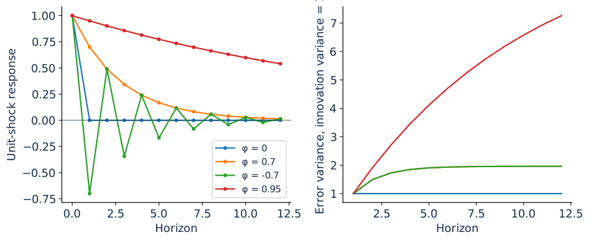
Persistence and forecast risk
Set persistence to −0.5. The response changes sign each period; the error variance keeps accumulating squared weights.
Values used in both graphs
| Horizon | Response, outcome units | Variance, squared units |
|---|---|---|
| 0 | 1.000000 | 0.000000 |
| 1 | 0.700000 | 1.000000 |
| 2 | 0.490000 | 1.490000 |
| 3 | 0.343000 | 1.730100 |
| 4 (selected) | 0.240100 | 1.847749 |
| 5 | 0.168070 | 1.905397 |
| 6 | 0.117649 | 1.933645 |
| 7 | 0.082354 | 1.947486 |
| 8 | 0.057648 | 1.954268 |
| 9 | 0.040354 | 1.957591 |
| 10 | 0.028248 | 1.959220 |
| 11 | 0.019773 | 1.960018 |
| 12 | 0.013841 | 1.960409 |
Original analytic teaching example. Parameters are known and innovation variance is one. These are conditional variances under conditional homoskedasticity; constant unconditional second moments support the same values as unconditional mean-squared errors.
Compare quarterly averaging with sampling every third month →
JavaScript enables the controls. The printed lecture includes the analytic curves and hand calculations.
Practice and laboratory for Lecture 2
- Assignment 2: Recursion and uncertainty, three tasks with worked answers.
- Run ch02 from the laboratory bundle in Python, R, or Julia.
- Interactive experiment: Persistence and forecast risk
- Lecture 2 summary, with the central equation, a problem, a failure, and its repair.