Time-Series Econometrics

Begin with a forecast someone must use

A regional electricity planner must choose a reserve for next month. An underprediction can leave insufficient capacity; an overprediction can commit expensive capacity that remains idle. The object of interest is neither an attractive fitted curve nor a coefficient with a small standard error. It is a decision made before next month’s demand is observed.

Write a sentence that names the decision, the target, the unit, and the clock. For this case: “At the end of month $t$, forecast the total megawatt-hours sold to residential customers in a specified state during month $t+1$, using the records available by the forecast date.” A change from residential sales to total generation changes the economic object. A change from a state to a utility service area changes the population. A change from the end of the month to the middle of the month changes the information available. Those changes belong in the specification before a model is selected.

Let $Y_{t+h}$ denote the target at horizon $h$, and let $\mathcal I_t$ denote the information available at the decision time. Under squared-error loss, the ideal forecast is

$$\widehat Y_{t+h|t}=\mathbb E[Y_{t+h}\mid\mathcal I_t].$$

This notation encodes a restriction. The forecast must be a function of $\mathcal I_t$. It cannot depend on an observation released tomorrow, even if that observation describes yesterday. The target date and the availability date are different attributes of a record.

We will use an argument ledger throughout the course. Each entry records a decision date, a target definition, the information admitted, the proposed model, the result that would count against it, and the action justified by the result. Begin the ledger before seeing a model comparison. Its purpose is to make changes in reasoning visible. A forecaster can revise a model; a forecaster cannot retroactively claim to have made the revised decision earlier.

Why conditional expectation solves this loss

Take any forecast $a$ measurable with respect to $\mathcal I_t$. Let $m=\mathbb E[Y\mid\mathcal I_t]$, temporarily suppressing the target subscript. Decompose the conditional expected loss:

$$\begin{aligned} \mathbb E[(Y-a)^2\mid\mathcal I_t] &=\mathbb E[(Y-m+m-a)^2\mid\mathcal I_t]\\ &=\operatorname{Var}(Y\mid\mathcal I_t)+(m-a)^2. \end{aligned}$$

The cross term vanishes because $\mathbb E[Y-m\mid\mathcal I_t]=0$. The first term does not depend on $a$. The second is minimized at $a=m$. This proves an optimality statement for a specified information set and a specified loss. It does not say a linear regression consistently estimates that conditional expectation, or that squared loss matches the planner’s actual costs.

The units also agree. If $Y$ is measured in MWh, $m$ and $a$ are in MWh; variance and squared loss are in MWh squared. An error reported in dollars cannot be compared directly with an error in MWh. A loss function that translates quantities into costs must specify that conversion.

Forecast errors obey an orthogonality condition. For any integrable $Z$ known at the decision date,

$$\mathbb E[(Y-m)Z]=0,$$

when the needed moments exist. Systematic errors correlated with an available predictor suggest information was left unused. Errors correlated with a future predictor need not reveal a feasible improvement. This difference will recur when we examine residual diagnostics and structural interpretations.

A series has more than one date

Represent a record as $(p,a,v,g,x)$: period described, availability date, vintage, geographic unit, and value. The latest published series usually selects the latest vintage for each period. A historical decision requires the vintage available at that earlier date. If GDP for quarter $p$ was first published in $p+1$ and subsequently revised, using the latest value at the old forecast origin changes both availability and measurement.

The course’s public teaching data are fixed extracts. Unless a dataset explicitly contains historical releases, it supports a pseudo-out-of-sample experiment on the downloaded vintage. Such an experiment respects the ordering of periods while retaining the values currently recorded for those periods. It does not reconstruct the complete information set of a historical forecaster. That qualification is a property of the data, not a defect that a better forecasting algorithm can remove.

The lecture’s release-clock example makes this distinction concrete. Periods are numbered from zero, and a record for period $p$ becomes available in period $p+2$. At decision date 8, period 6 is the latest available observation. A training sample through period 8 would include two unreleased records. The code filters on release <= origin before selecting the latest period. In an applied project, dates replace the integers, but the rule is identical.

A valid forecasting table should retain origin, target_period, available_through, model_version, forecast, and, once observed, actual. Joining predictions to actuals by row position is unsafe after missing months or revisions. Join by explicit target identifiers and check that every forecast precedes the target’s availability.

Geographic aggregation changes the variable

Suppose a state has two areas with temperatures $40^\circ F$ and $80^\circ F$, and equal weights. Its mean temperature is $60^\circ F$. Define heating degree days relative to $65^\circ F$ as $H(T)=\max(65-T,0)$. Transforming the state mean produces $H(60)=5$. Transforming each area first and averaging produces $(H(40)+H(80))/2=12.5$.

$$H\!\left(\sum_i w_iT_i\right)\ne\sum_iw_iH(T_i).$$

Here the inequality follows from the kink in $H$. More generally, Jensen’s inequality gives $H(\mathbb E[T])\leq\mathbb E[H(T)]$ because $H$ is convex. Aggregating first erases some exposure to cold locations. The course code returns 5 and 12.5 from the same temperature observations. This is an exact arithmetic example, independent of sampling error.

Weights must also represent an economic object. Population weights approximate exposure of people; electricity-customer weights approximate exposure of customers; geographic area weights approximate exposure of land. None is automatically the right measure of electricity demand. If weights change over time, a change in the index can reflect changing composition as well as changing temperatures. Retaining fixed weights answers a different question from updating them.

A useful measurement specification names the source locations, inclusion rules, units, weights, missing-value treatment, and transformation order. Boundary changes require a crosswalk or a declared break. A station average should not silently become a population-weighted state measure. This is where geographic econometrics enters the course: the geography determines the observed variable before a temporal model is fitted.

Establish a benchmark before adding complexity

For a persistent level, the naive forecast is $\widehat Y_{t+1|t}=Y_t$. For a monthly seasonal series, the seasonal naive forecast is $\widehat Y_{t+h|t}=Y_{t+h-12k}$, where $k$ is the smallest positive integer making the referenced month available. For a series with a stable mean, a training-sample mean can be another benchmark. These are different economic assumptions expressed as forecast rules.

The naive forecast assumes that the last level is a useful anchor. The seasonal naive forecast assumes the same calendar month of the prior year is a useful anchor. A historical mean assumes the relevant mean has remained stable. Benchmarks can fail; the point of specifying them is to know what a complicated model improves upon.

Do not choose a benchmark after seeing which one makes your preferred model look best. Record the benchmark and loss in the ledger, then hold them fixed through the first comparison. If the economic target later changes, open a new comparison with a stated reason.

The synthetic series in this lecture is $Y_t=100+X_t$, where $X_t=0.8X_{t-1}+\varepsilon_t$. Its units are teaching units, not observed electricity sales. The executable example evaluates the naive forecast on the final 60 targets. Run the same shared fixture in each language; the reported root mean squared error should agree to numerical tolerance. We will add an estimated autoregression and a matched forecast-origin comparison in Lecture 4.

Execute, break, and repair

Download the complete laboratory bundle, extract it, and open a terminal in its code directory. In Python, run uv sync --locked once and then uv run python ch01.py; in R, run Rscript ch01.R; in Julia, run julia --startup-file=no ch01.jl. The code page lists the tested versions. Each entry point calls the implementation in the corresponding course file and cannot run outside that directory. All implementations read the same innovations.csv. The file contains simulated shocks generated by a documented algorithm; it is not a sample of observed economic outcomes.

Before running, predict the latest available period and both heating-degree-day measures. Record your predictions. After running, inspect the transformation order in the source. Then replace the availability filter release <= origin with the period filter period <= origin. Periods 7 and 8 enter the training rows, and the code’s audit, which looks up each included record’s own release date and asserts that it is at most the origin, fails. Restore the availability filter and confirm that the audit passes with seven included records. An assertion that only restates the filter it is meant to check could never fail; this one compares each selected row with its own release date, whichever filter selected it.

Next alter the geographic weights from $(0.5,0.5)$ to $(0.8,0.2)$. Compute both orders of transformation by hand. The weighted temperature becomes $48^\circ F$, its heating degree days become 17, and the weighted local heating measure becomes 20. The direction of Jensen’s inequality remains unchanged. The size of the discrepancy changes because the economic weights changed.

Practice with a worked answer

A monthly observation describes March, is released May 10, and is revised July 15. A forecast is issued May 1. Can the forecaster use the first release? Can a retrospective analyst use the July vintage to claim a real-time May 1 forecast?

The first answer is no: May 10 follows May 1. The second answer is also no: the July value was unavailable at the original decision date. The analyst can run a retrospective experiment using the July vintage, provided that experiment is labeled accordingly. To reconstruct a real-time forecast, the analyst needs the records actually available on May 1, possibly ending before March.

Now suppose monthly electricity sales are a flow and end-of-month installed capacity is a stock. How should a quarterly series be formed? Sum the three monthly sales flows. Use an explicitly defined quarter-end capacity stock, or an average stock if the question concerns average capacity during the quarter. Summing three installed-capacity stocks would count the same equipment repeatedly and change the quantity’s meaning.

Your ledger entry should now state a target, a release rule, a geographic definition, a benchmark, and one result that would force revision. Keep this entry for Project 1. The next lecture will replace the benchmark’s implicit dynamics with a model whose behavior we can derive.

Sources and further reading

The EIA-861M data documentation defines electricity sales, sectors, and state adjustments. The NOAA Climate at a Glance documentation describes geographic climate series. The forecasting distinction between training residuals and test errors is developed in Forecasting: Principles and Practice, Section 5.8.

A model for a persistent economic level

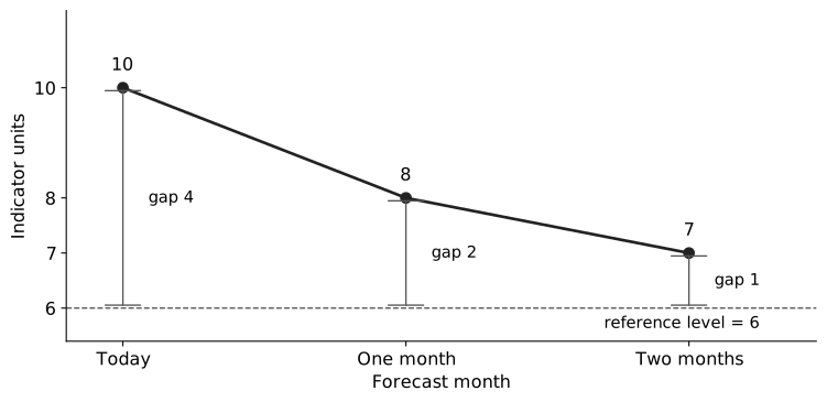
Suppose a monthly economic indicator is 10 today. We need a forecast for the next two months. Our model adds 3 each month and carries forward half the previous value. With no new shock, next month’s value is $3+0.5\times10=8$. One month later it is $3+0.5\times8=7$.

Why does the forecast move down? A value of 6 reproduces itself: $3+0.5\times6=6$. Today the indicator is 4 units above that level. One step leaves half the gap; two steps leave a quarter. We can therefore calculate the same two-month forecast as $6+0.5^2(10-6)=7$. These are invented numbers for a hand calculation; they are not estimates for the Texas electricity case.

Now write the rule as

$$Y_t=c+\phi Y_{t-1}+\varepsilon_t, \qquad \mathbb E[\varepsilon_t\mid\mathcal I_{t-1}]=0, \qquad\mathbb E[\varepsilon_t^2]=\sigma^2.$$

The model is an autoregression of order one, abbreviated AR(1). Here $c=3$ and $\phi=0.5$. The coefficient $\phi$ describes how much of a deviation survives one period. The intercept $c$ is the increment in the recursion; the reference level is $c/(1-\phi)$ when $|\phi|<1$. The innovation $\varepsilon_t$ is what the previous information could not predict. Its zero conditional mean lets the calculations above serve as forecasts even though future shocks will usually be nonzero.

The conditional-mean restriction rules out predictable innovations. Serially uncorrelated errors alone do not imply independence, Gaussianity, or this restriction. The second moment displayed above is unconditional: it averages across histories. It does not require the risk faced at each history to be the same. We will state the stronger condition when we calculate a conditional forecast variance. Treat $c$ and $\phi$ as known until the section on estimation uncertainty.

Here $\mathcal I_t$ contains the observations and innovations through $t$; these information sets grow as records arrive. The known recursion lets us recover an observed innovation as $Y_t-c-\phi Y_{t-1}$. All innovations have finite second moments. These conditions make the conditioning steps below meaningful.

Lecture 1’s conditional-expectation proof explains why averaging the unknown future given today’s information minimizes squared forecast loss. Here we apply that result to a specific recursion.

If $Y$ is in MWh, $c$ and $\varepsilon$ are in MWh and $\phi$ is dimensionless. The interval represented by one time step matters. A monthly persistence coefficient cannot be substituted directly into a quarterly recursion.

Solve the difference equation

Substitute the recursion repeatedly:

$$Y_t=\phi^tY_0+c\sum_{j=0}^{t-1}\phi^j+ \sum_{j=0}^{t-1}\phi^j\varepsilon_{t-j}.$$

To see the pattern, the first substitution gives $Y_2=\phi^2Y_0+c(1+\phi)+\phi\varepsilon_1+\varepsilon_2$. One more substitution multiplies every existing term by $\phi$, then adds $c+\varepsilon_3$. Thus a shock from $j$ periods ago receives exactly $j$ multiplications by $\phi$.

The finite geometric sum also has a short proof. Write $S_t=1+\phi+\cdots+\phi^{t-1}$. Subtract $\phi S_t=\phi+\cdots+\phi^t$ from it; all interior terms cancel, leaving $(1-\phi)S_t=1-\phi^t$. Hence $S_t=(1-\phi^t)/(1-\phi)$ when $\phi\ne1$. At $\phi=1$, each term equals one and $S_t=t$.

For $\phi\ne1$, the deterministic component is $\phi^tY_0+c(1-\phi^t)/(1-\phi)$. If $|\phi|<1$, the initial condition’s influence decays. Under the finite-moment conditions specified next, a stationary solution can be written

$$Y_t=\mu+\sum_{j=0}^{\infty}\phi^j\varepsilon_{t-j}, \qquad \mu=\frac{c}{1-\phi}.$$

For this representation, let the innovation sequence extend through all integer dates, with zero means, common variance $\sigma^2$, and zero covariances across distinct dates. The mean-square size of the omitted tail after $m$ terms is $\sigma^2\sum_{j=m}^{\infty}\phi^{2j}$, which tends to zero when $|\phi|<1$. That establishes mean-square convergence. The resulting mean is constant and its covariance depends only on the lag, so the solution is covariance-stationary. Strict stationarity, which concerns the entire joint distribution, requires a strictly stationary innovation sequence as well.

A simulation initialized at an arbitrary fixed $Y_0$ has a transient; it is not exactly stationary from its first row. Discarding a burn-in approximates the covariance-stationary regime, with approximation quality depending on persistence.

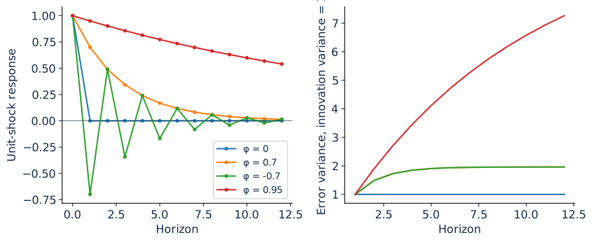
For $\phi=0$, each observation is $c+\varepsilon_t$. For $0<\phi<1$, deviations decay without alternating signs. For $-1<\phi<0$, their signs alternate while their magnitudes decay. At $\phi=1$, the formula for $\mu$ is undefined and the model becomes a random walk with drift. For $|\phi|>1$, the forward recursion is explosive. Those boundary cases should change an implementation’s interpretation, not merely trigger a divide-by-zero warning.

Derive the population moments

Taking expectations in a stationary solution yields $\mu=c+\phi\mu$, hence $\mu=c/(1-\phi)$. Subtract the mean and define $X_t=Y_t-\mu$. Then

$$X_t=\phi X_{t-1}+\varepsilon_t.$$

The previous state is known in $\mathcal I_{t-1}$, so $\mathbb E[X_{t-1}\varepsilon_t]=\mathbb E[X_{t-1}\mathbb E[\varepsilon_t\mid\mathcal I_{t-1}]]=0$. Squaring the centered recursion and taking expectations therefore gives

$$\gamma(0)=\phi^2\gamma(0)+\sigma^2.$$

Stationarity supplies the same variance for $X_t$ and $X_{t-1}$. Subtract $\phi^2\gamma(0)$ from both sides and divide by $1-\phi^2$, which is positive for $|\phi|<1$: $\operatorname{Var}(Y_t)=\gamma(0)=\sigma^2/(1-\phi^2)$.

Define $\gamma(k)=\mathbb E[X_tX_{t-k}]$. Multiply the centered recursion by $X_{t-k}$ and take expectations. For $k\ge1$, $X_{t-k}$ is known before the innovation, so the same conditioning argument makes its product with $\varepsilon_t$ contribute zero. The remaining product is $\phi\mathbb E[X_{t-1}X_{t-k}]=\phi\gamma(k-1)$ by stationarity. Iterating gives

$$\gamma(k)=\phi^k\gamma(0),\qquad\rho(k)=\phi^k.$$

Covariance has squared outcome units. Correlation and persistence are dimensionless. As $|\phi|$ approaches one with $\sigma^2$ held fixed, stationary variance grows without bound. A small innovation variance therefore does not guarantee a stable level. Negative persistence gives alternating correlations, while variance depends on $\phi^2$.

The laboratory uses $c=0.6$, $\phi=0.7$, and $\sigma^2=1$. Its population mean is 2 and population variance is approximately 1.9608. The simulated sample will differ. That discrepancy is evidence of finite-sample variation; it should not be repaired by changing the population formulas to match the realized sample.

Comparing a time average with a population moment needs one more condition, because stationarity alone does not make time averages converge. Draw $Z$ once and let $Y_t=Z+\varepsilon_t$ with independent innovations. The process is strictly stationary, yet its sample mean converges to the realized $Z$ rather than to $\mathbb E[Y_t]$: one long history reveals nothing about the other values $Z$ could have taken. The missing property is ergodicity, under which time averages of functions of the process converge to their expectations. For a strictly stationary process, a sufficient condition is mixing, under which events far apart in time become asymptotically independent. For the sample mean of a stable AR(1), less is needed. Under the linear-process assumptions above, the autocovariances are absolutely summable, so $\operatorname{Var}(\overline Y)\to0$ and $\overline Y$ converges in mean square to $\mu$. Sample variances, autocovariances, and the least-squares estimators of later lectures need more, such as independent innovations with finite variance, martingale-difference innovations with suitable higher moments, or a mixing condition that supports a law of large numbers and a central limit theorem for dependent data. Later laboratories assume conditions of this kind whenever they treat a time average as an estimate.

Forecast more than one period ahead

At date $t$, iterate the centered recursion forward:

$$Y_{t+h}=\mu+\phi^h(Y_t-\mu) +\sum_{j=0}^{h-1}\phi^j\varepsilon_{t+h-j}.$$

Under the innovation conditional-mean restriction, the forecast is

$$\widehat Y_{t+h|t}=\mu+\underbrace{\phi^h(Y_t-\mu)}_{\text{retained deviation}}.$$

Each future innovation has zero conditional mean given date-$t$ information: condition first on the information immediately before that innovation, use its zero conditional mean, then condition on $\mathcal I_t$. That removes it from the forecast, but its squared contribution remains in the error. The same conditioning argument makes the cross-products of innovations at different dates vanish.

Take two future dates $t<i<k$. The earlier innovation is already known in $\mathcal I_{k-1}$, and $\mathcal I_t$ is contained in that information set. Conditional expectation therefore gives

$$\mathbb E[\varepsilon_i\varepsilon_k\mid\mathcal I_t] =\mathbb E[\varepsilon_i\mathbb E[\varepsilon_k\mid\mathcal I_{k-1}]\mid\mathcal I_t]=0.$$

The inner expectation is zero by the model’s innovation restriction. Averaging the resulting zero over the histories also gives an unconditional zero cross-product. Expand the squared forecast error: the cross-terms disappear, leaving each innovation’s second moment multiplied by its squared coefficient. With the common unconditional second moment $\sigma^2$, this yields the unconditional mean-squared forecast error

$$V_h=\sigma^2\sum_{j=0}^{h-1}\phi^{2j} =\sigma^2\frac{1-\phi^{2h}}{1-\phi^2}.$$

For this same number to be the conditional forecast variance at every history, assume conditional homoskedasticity: $\mathbb E[\varepsilon_s^2\mid\mathcal I_{s-1}]=\sigma^2$ for the future dates involved. The word means that the next innovation’s variance is constant given the available history. Without that condition, the conditional variance instead sums $\phi^{2j}\mathbb E[\varepsilon_{t+h-j}^2\mid\mathcal I_t]$ over $j=0,\ldots,h-1$. The forecast mean can remain correct while its conditional risk changes.

For $h=1$, $V_h=\sigma^2$. For a stable process, it increases toward the unconditional level variance. At $\phi=1$, use the finite sum directly: $V_h=h\sigma^2$. Numerical cancellation near one can make the quotient less accurate than the sum.

With the opening example’s $\phi=0.5$ and innovation standard deviation 2, the two-month error is $0.5\varepsilon_{t+1}+\varepsilon_{t+2}$. Under conditional homoskedasticity its variance is $0.5^2\times4+4=5$ squared indicator units. Changing $\phi$ to $-0.5$ reverses the first innovation’s contribution but leaves its squared weight at $0.25$. The response can alternate while the variance remains positive. Change persistence and compare both quantities.

A changed example: what if risk depends on the history?

An observed risk state chooses an innovation scale of 1 or 3, each with probability one half, and retains that scale over the two forecast months. Each month’s innovation is the scale times an independent sign, equally likely to be $-1$ or $1$. What are the two conditional error variances when $\phi=0.5$? What is their unconditional average?

In the low-risk state, variance is $1^2(1+0.5^2)=1.25$. In the high-risk state it is $3^2(1+0.5^2)=11.25$. Their average is $6.25$, which also equals $\mathbb E[\varepsilon_s^2](1+0.5^2)=5\times1.25$. Zero conditional means and constant unconditional second moments hold, but conditional homoskedasticity fails. Reporting 6.25 as the risk at either observed history would be wrong. The independent signs permit an exact eight-outcome enumeration across the two risk states; no simulation is needed for this example.

A shock’s response after $h$ periods is $\phi^h$ times its initial size. For $0<\phi<1$, solving $\phi^h=0.5$ gives the half-life $\log(0.5)/\log(\phi)$. This is a real-valued number of model periods; actual discrete responses reach or fall below half their original magnitude at the ceiling of that number. For $-1<\phi<0$, use $|\phi|$ to describe magnitude decay and retain the alternating sign separately.

The known-parameter variance excludes parameter uncertainty. When $c$ and $\phi$ are estimated, a plug-in forecast is a random function of an estimated model. Its interval requires additional care, especially in a short sample or near a unit root. Lecture 4’s forecast-uncertainty discussion distinguishes process uncertainty, estimation uncertainty, and uncertainty about model selection.

Time aggregation changes the dependence

Suppose a monthly centered AR(1) is observed only through quarterly averages

$$Q_s=\frac{X_{3s-2}+X_{3s-1}+X_{3s}}3.$$

Using $\gamma(k)=\gamma(0)\phi^{|k|}$,

$$\operatorname{Var}(Q_s)=\frac{\gamma(0)}9(3+4\phi+2\phi^2).$$

There are three diagonal covariance terms, four ordered pairs at distance one, and two at distance two. Between adjacent quarters, the nine pairwise distances are 1, 2, 2, 3, 3, 3, 4, 4, and 5. Thus

$$\operatorname{Cov}(Q_s,Q_{s-1}) =\frac{\gamma(0)}9(\phi+2\phi^2+3\phi^3+2\phi^4+\phi^5).$$

Their ratio is generally different from $\phi^3$. Sampling the last month of each quarter produces a different dependence structure from averaging all three months. The aggregate process can require moving-average terms even when the original process is a simple autoregression. This is a substantive measurement issue: the model belongs to the frequency and aggregation rule actually used.

For a quarterly flow total, replace the average by a sum. Variance and covariance both multiply by nine, leaving the correlation unchanged. The level’s units change from a monthly quantity to a quarterly total, so its intercept and forecast scale change. A rate or index may instead require an economically defined weighted average.

Execute the recursion and audit the result

Run ch02 in your preferred language. The source implements the recursion directly and computes the four-step forecast twice: by applying the recursion four times to the last observation, and by the closed formula $\mu+\phi^4(Y_t-\mu)$. It asserts that the two agree to $10^{-12}$ and reports both. The same program compares the finite variance sum with its quotient and asserts numerical agreement, and it averages consecutive groups of three monthly observations to estimate an AR(1) coefficient on that aggregate.

First predict whether that aggregate coefficient should equal $0.7^3$. Use the covariance expressions above to explain your prediction. Compare the realized estimate with the implied aggregate lag-one correlation; finite samples and the fitted intercept will introduce differences. A single sample is a demonstration, not a consistency proof.

Then repeat the recursion at $\phi=0$, $0.95$, $-0.7$, and $1$. At one, retain the finite forecast-error sum and stop reporting a stationary population mean. At $0.95$, increase the burn-in and explain why the shorter burn-in retained more initial-condition influence. The code’s baseline burn-in is an explicit design choice, not a universal guarantee.

Worked problem and project connection

Return to the opening example with $c=3$, $\phi=0.5$, innovation standard deviation 2, and current value 10. Its stationary mean is 6 and its two-period forecast is 7. Under conditional homoskedasticity, its known-parameter conditional error variance is 5 and its standard deviation is $\sqrt5$. If the future innovations are independent Gaussian draws, the conditional Gaussian 95% interval is $7\pm1.96\sqrt5$. Using 1.96 rounds the normal quantile; variance alone does not justify a Gaussian interval.

If the current value changes from 10 to 14, the two-period forecast increases by $0.5^2(4)=1$. The error variance is unchanged because this homoskedastic model makes variance independent of the current level. If observed forecast risk increases with the level, this model’s variance assumption deserves an audit.

In Project 1: A forecast someone can use, use an AR model as a transparent competitor to the benchmark. Report the series frequency, its aggregation rule, fitted persistence, and the estimation window. Describe which disturbance remains unexplained. The next lecture will expand the dependence structure while preserving the distinction between observable histories and unobserved innovations.

Further reading

For the transition from independent Gaussian shocks to the weaker zero-conditional-mean condition, see QuantEcon’s discussion of martingale difference shocks. Its prediction section develops the state-space generalization. The ARIMA chapter in Forecasting: Principles and Practice supplies forecasting context. The numerical examples and graphics in this lecture are original teaching calculations.

Separate propagation from innovation memory

An autoregression propagates past outcomes. A moving-average model carries past innovations into the current observation. For a centered series, an ARMA(1,1) combines both:

$$X_t=\phi X_{t-1}+\varepsilon_t+\theta\varepsilon_{t-1}.$$

Our convention places a plus sign before $\theta$. Software packages and textbooks sometimes use different signs. Record the convention before comparing estimates. A coefficient disagreement caused by opposite conventions is a notation mismatch, not an empirical contradiction.

Define the lag operator $LX_t=X_{t-1}$. The model is $(1-\phi L)X_t=(1+\theta L)\varepsilon_t$. A general ARMA$(p,q)$ has

$$\Phi(L)X_t=\Theta(L)\varepsilon_t, \quad \Phi(z)=1-\sum_{i=1}^p\phi_i z^i, \quad\Theta(z)=1+\sum_{j=1}^q\theta_jz^j.$$

For a causal stationary representation, the roots of $\Phi(z)=0$ must lie outside the unit circle. For an invertible innovation representation, the roots of $\Theta(z)=0$ must lie outside it. These conditions concern different polynomials and different questions. For ARMA(1,1), they become $|\phi|<1$ and $|\theta|<1$, respectively.

Build the moving-average representation

When $|\phi|<1$,

$$X_t=\frac{1+\theta L}{1-\phi L}\varepsilon_t =\sum_{j=0}^{\infty}\psi_j\varepsilon_{t-j},$$

where $\psi_0=1$ and $\psi_j=(\phi+\theta)\phi^{j-1}$ for $j\ge1$. Obtain the coefficients by multiplying $(1+\theta L)$ by $\sum_{j\ge0}\phi^jL^j$. This representation shows the immediate innovation effect and the later propagation effects.

With serially uncorrelated innovations of variance $\sigma^2$,

$$\gamma(0)=\sigma^2\sum_{j\ge0}\psi_j^2 =\sigma^2\frac{1+\theta^2+2\phi\theta}{1-\phi^2}.$$

The numerator and denominator are dimensionless, leaving squared outcome units. At $\theta=0$, this reduces to the AR(1) variance. At $\phi=0$, it becomes $\sigma^2(1+\theta^2)$, the MA(1) variance. At $\theta=-\phi$, the lag polynomials cancel and $X_t=\varepsilon_t$. Such common factors make an unnecessarily large model observationally redundant.

The lag-one covariance is

$$\gamma(1)=\phi\gamma(0)+\theta\sigma^2.$$

Multiply the original recursion by $X_{t-1}$ and take expectations. The current innovation is uncorrelated with the past, while $\operatorname{Cov}(\varepsilon_{t-1},X_{t-1})=\sigma^2$. For $k\ge2$, $\gamma(k)=\phi\gamma(k-1)$. The first lag therefore contains both autoregressive propagation and moving-average memory; later lags decay geometrically.

Why invertibility matters

For an MA(1), $X_t=\varepsilon_t+\theta\varepsilon_{t-1}$. If $|\theta|<1$,

$$\varepsilon_t=(1+\theta L)^{-1}X_t =\sum_{j=0}^{\infty}(-\theta)^jX_{t-j}.$$

The coefficients decay, so distant observations have diminishing influence on the recovered innovation. If $|\theta|>1$, this backward recursion amplifies initialization error. A stable series can therefore have a noninvertible representation: stationarity does not guarantee stable recovery of shocks from observed history.

The MA(1) autocorrelation is $\rho(1)=\theta/(1+\theta^2)$ and $\rho(k)=0$ for $k>1$. Replacing $\theta$ by $1/\theta$ preserves $\rho(1)$. It also preserves the covariance function if the innovation variance is rescaled to $\theta^2\sigma^2$. Gaussian processes with these matched covariance functions have the same distribution. An invertibility convention selects the representation with recoverable innovations; the ACF alone cannot distinguish reciprocal MA roots.

This does not mean all non-Gaussian models with the same covariance are identical in every respect. Covariance characterizes second-order behavior; additional distributional information can matter. Our elementary identification statement should remain within its assumptions.

Read an ACF and PACF without treating them as verdicts

The autocorrelation function measures the association between $X_t$ and $X_{t-k}$. The partial autocorrelation at lag $k$ removes linear dependence on the intervening $k-1$ lags. Equivalently, it is the final coefficient in the population linear projection of $X_t$ onto its first $k$ lags under the usual nonsingularity conditions.

For a pure AR$(p)$, the population PACF cuts off after $p$ and the ACF generally tails off. For a pure MA$(q)$, the population ACF cuts off after $q$ and the PACF generally tails off. For a mixed ARMA, both can tail off. Seasonal dynamics introduce patterns at seasonal lags. Differencing, finite samples, parameter cancellation, and near-unit roots complicate these pictures.

An estimated ACF is noisy. A familiar $\pm1.96/\sqrt n$ band is a rough white-noise reference, not a simultaneous confidence band for every lag of every fitted model. Inspecting many lags creates many opportunities for an apparent excursion. Use the plots to propose a short candidate list, then check residuals and evaluate the candidates on later targets.

Information criteria rank such a list. For a Gaussian model with $k$ estimated parameters fitted to $n$ observations, and up to terms common to every candidate,

$$\operatorname{AIC}=n\log\widehat\sigma^2+2k,\qquad \operatorname{BIC}=n\log\widehat\sigma^2+k\log n,$$

where $\widehat\sigma^2$ is the estimated innovation variance (Akaike 1974; Schwarz 1978). The preferred candidate minimizes the criterion. BIC’s penalty exceeds AIC’s once $n\ge8$, so BIC chooses smaller models. When the true orders are among the candidates, BIC selects them with probability approaching one, while AIC retains a positive probability of overfitting; AIC is designed instead to approximate expected predictive loss. Compute every criterion on a common estimation sample, because a model with more lags loses initial observations, and criteria computed on different samples are not comparable. Select the order inside the training window and treat that selection rule as part of the procedure that later targets evaluate.

The laboratory’s ARMA series has $\phi=0.6$ and $\theta=0.4$. Its sample lag-one correlation is substantially larger than the isolated MA(1) correlation $0.4/(1+0.4^2)$. Comparing those two values does not reveal an error: one belongs to a mixed model and the other to a pure MA benchmark. Calculate the mixed-model population correlation using the formulas above before interpreting the sample.

Estimate a conditional model transparently

Given a candidate $(\phi,\theta)$ and an initialization $\widehat\varepsilon_0=0$, recover residuals recursively:

$$\widehat\varepsilon_t =X_t-\phi X_{t-1}-\theta\widehat\varepsilon_{t-1}.$$

Conditional sum of squares minimizes $\sum_t\widehat\varepsilon_t^2$. The source uses a small declared grid and excludes the first 30 residuals from the comparison. A grid estimate is transparent but coarse. It supplies neither exact maximum likelihood nor standard errors. Its pedagogical purpose is to expose the objective, initialization, parameter restrictions, and residual recursion before using a package optimizer.

When fitting real data, an exact Gaussian likelihood accounts for the initial state distribution; conditional likelihood conditions on initial information. Near boundaries, small-sample estimates can depend appreciably on that treatment. An optimizer’s successful exit does not prove the global optimum or the economic validity of the model. Retain its convergence information and inspect admissibility.

Estimate a mean explicitly, or center using training data only. Centering with the full sample before forecasting leaks future information into the historical regressors. The lecture’s synthetic ARMA is constructed with zero mean, so its grid search has no estimated mean term. That simplifying assumption must not silently migrate to an application with a changing level.

Execute, break, and repair

Run ch03 in all three languages. The declared grid includes the generating coefficients, and the shared realization selects them under the conditional criterion. The code records the conditional mean squared residual at all sixteen grid points. The minimum, 0.939 at $(\phi,\theta)=(0.6,0.4)$, is close to its neighbors 0.991 at $(0.8,0.4)$ and 1.010 at $(0.4,0.4)$, while $(0.6,-0.4)$ gives 1.693. Use the grid to judge how sharply the objective distinguishes nearby candidates. Recover the residuals, then calculate their ACF. A model that reproduces the outcome’s ACF can still leave predictable residual patterns.

Set $\theta=1.2$ in the data generator and try the innovation recursion with that coefficient. Perturb the initial residual by a small amount. The initialization difference evolves as $(-\theta)^t$ and grows in magnitude. Repeat at $\theta=0.4$; the difference decays. Repair the representation by finding the reciprocal invertible coefficient and rescaling innovation variance. Explain which features of the observed series are retained.

Next set $\theta=-\phi$. The simulated series collapses to white noise apart from initialization handling. A two-parameter model that seems flexible here is redundant. Simplify the representation and record the reason in the ledger.

Worked problems

For an MA(1) with $\theta=0.5$ and $\sigma^2=4$, variance is $4(1+0.25)=5$ and lag-one covariance is $0.5(4)=2$. Thus $\rho(1)=0.4$. The reciprocal representation has coefficient 2 and innovation variance 1; its variance is again 5 and its lag-one covariance again 2. The first representation is invertible; the second is not.

For an ARMA(1,1) with $\phi=0.5$, $\theta=0.2$, and $\sigma^2=1$, variance is $(1+0.04+0.2)/(1-0.25)=1.653\overline3$. Lag-one covariance is $0.5(1.653\overline3)+0.2=1.026\overline6$, giving lag-one correlation approximately 0.621. Lag-two covariance is half the lag-one covariance. These checks establish the correct sign convention before any software result is interpreted.

For Project 1, declare a small candidate family and justify it through the target’s dynamics. Preserve the benchmark, information rule, and forecast origins. A larger model earns its place through a defensible improvement on that comparison. Lecture 4 specifies the comparison itself.

Further reading

QuantEcon’s ARMA lecture develops covariance-stationary processes in time and frequency domains. Forecasting: Principles and Practice discusses practical ARIMA model selection.

Fitting and forecasting answer different questions

A regression’s fitted values use coefficients estimated from its training sample. Their residuals describe how that fitted model represents observations it has already seen. A forecast uses a model constructed before its target is observed. Its errors describe performance on subsequent targets. A small training residual sum of squares can coexist with poor forecasting.

Begin with a historical sequence and a forecast origin $t$. The training window ends at that origin, or at the latest earlier observation available under the release rule. Fit the model using only that window, issue a forecast for $t+h$, and retain the prediction. Move the origin forward and repeat. This is rolling-origin evaluation. An expanding window starts at a fixed initial date; a rolling window retains a fixed number of recent observations.

An honest comparison holds the target periods, information rule, and loss fixed across methods. If one model is evaluated only on easy months and another on every month, their average losses are not comparable. If a model cannot produce a forecast at an origin, record that failure and apply a declared fallback rule. Do not silently drop the difficult target.

The comparison should reflect the intended deployment. Refitting at every origin evaluates a repeatedly updated procedure. Fitting once and holding coefficients fixed evaluates a different procedure. Both are legitimate designs if their interpretation is explicit.

The algorithm is part of the statistical model

For an estimated AR(1), the procedure at each origin solves

$$\min_{c,\phi}\sum_{s\in W_t}(Y_s-c-\phi Y_{s-1})^2,$$

then iterates the estimated recursion $h$ steps. $W_t$ contains admissible target-regressor pairs from that origin’s training window. A lagged outcome requires both rows to be available; missing periods must not turn adjacent rows into a false one-period lag.

The executable implementation uses QR-based least squares. Solving the normal equations by explicitly inverting $X'X$ is unnecessary and can amplify numerical problems. Rank checks detect a design with redundant columns or insufficient observations. This is a computational condition; rank sufficiency does not establish exogeneity, stationarity, or stability. Whether the estimated $c$ and $\phi$ approach their population values as the training window grows is a statistical question, and the answer rests on stability together with the ergodicity and innovation conditions stated in Lecture 2.

Preprocessing also belongs inside the origin loop. Estimate a mean, standard deviation, imputation rule, seasonal adjustment, or principal component from training data. Apply the retained transformation to the admissible prediction inputs. A full-sample transformation can carry information from the test period into every historical forecast even when the regression itself is refitted correctly.

Tuning requires another boundary. Use an earlier validation segment to choose lag order or window length, then evaluate the chosen procedure on later targets. Repeatedly choosing a model after observing the same test errors turns that test segment into a selection sample. Lecture 14 will freeze a complete procedure before a continuation release.

Match loss to the decision

For errors $e_t=Y_t-\widehat Y_t$, common summaries are

$$\operatorname{MAE}=\frac1n\sum_t|e_t|, \qquad \operatorname{RMSE}=\sqrt{\frac1n\sum_te_t^2}.$$

Both are in outcome units. RMSE emphasizes large errors. MAE has the conditional median as its population-optimal point forecast; squared loss has the conditional mean. Percentage errors are problematic near zero and can compare series in economically misleading ways. For a scaled error, calculate its scaling denominator from the training sample and state the benchmark defining that scale.

If underprediction costs $c_u$ per unit and overprediction costs $c_o$, define

$$L(a,Y)=c_u(Y-a)_++c_o(a-Y)_+.$$

For a continuous conditional distribution $F$, differentiating expected loss with respect to $a$ gives $-c_u[1-F(a)]+c_oF(a)$. The optimum satisfies

$$F(a)=\frac{c_u}{c_u+c_o}.$$

With $c_u=3$ and $c_o=1$, the preferred action is the conditional 75th percentile. An unbiased conditional-mean forecast can therefore be an inappropriate reserve decision. The distinction is between estimating an outcome distribution and choosing an action from that distribution.

Identify the uncertainty in an interval

For a known-parameter stable AR(1), the $h$-step process variance is $V_h=\sigma^2\sum_{j=0}^{h-1}\phi^{2j}$. Gaussian innovations give a conditional Gaussian forecast distribution, so an interval is $\widehat Y\pm z_{1-\alpha/2}\sqrt{V_h}$.

There are several practical qualifications. Estimating parameters adds uncertainty; selecting a model adds another layer; a future covariate may need its own forecast; a geographic measure may be uncertain; and a structural break can invalidate the fitted process entirely. A normal interval computed from a residual variance addresses only the assumptions included in that calculation.

One possible approximation for a one-step regression forecast adds the coefficient-estimation term:

$$\widehat\sigma^2\left[1+x_{t+1}'(X'X)^{-1}x_{t+1}\right].$$

This formula assumes the usual homoskedastic regression conditions and treats the prediction regressors appropriately. It is not a universal ARMA multi-step interval. With dependence, a simulation or bootstrap should preserve the relevant temporal structure and repeat the actual fitting procedure. Resampling individual time rows indiscriminately destroys that structure.

Check intervals empirically. Record coverage, average width, and behavior in periods relevant to the decision. High coverage from enormous intervals can be operationally unhelpful. Narrow intervals with severe undercoverage misstate risk. For overlapping multi-step targets, successive errors are dependent, so a binomial standard error is generally inappropriate without addressing that dependence.

Compare paired errors

Let $e_{A,t}$ and $e_{B,t}$ be errors on identical targets. Analyze

$$d_t=L(e_{A,t})-L(e_{B,t}).$$

A negative mean favors A for that loss and those targets. Pairing preserves the fact that both forecasts face the same difficult months. A standard error for $\overline d$ must reflect serial dependence, including dependence from overlapping horizons and repeated estimation. A heteroskedasticity-and-autocorrelation-consistent estimate or a carefully designed block bootstrap can be suitable under its assumptions.

The ratio $\overline d/\widehat{\operatorname{se}}(\overline d)$ is the test of equal predictive accuracy proposed by Diebold and Mariano (1995), who treated the two forecast sequences as given. For $h$-step forecasts, $d_t$ inherits the MA$(h-1)$ dependence of overlapping errors described in the diagnostics section below, so the HAC estimate should include at least $h-1$ lags. When a forecast is misspecified, as the no-change forecast is for the stationary AR(1) in this lecture’s laboratory, its errors and $d_t$ can be dependent beyond lag $h-1$, and $h-1$ lags is then only a lower bound. The Bartlett weights of Newey and West (1987) keep the estimate nonnegative.

Forecasts from estimated models add a complication. West (1996) showed that parameter estimation can contribute a term to the asymptotic variance of $\overline d$. His results require that variance to be positive, and that requirement fails when one model nests the other, which is the case in this lecture: the no-change forecast is the AR(1) with $c=0$ and $\phi=1$. Under the null of equal population accuracy, the two nested forecasts coincide in population, the loss differential degenerates, and the DM statistic does not have a standard normal limit. Clark and McCracken (2001) and McCracken (2007) derive nonstandard critical values for such comparisons. Giacomini and White (2006) pose a different null: whether two forecasting methods, each including its estimation window, have equal expected loss given the information available at the origin. With an estimation window of fixed length, their test uses normal or chi-squared critical values for nested and non-nested models alike. An expanding window lies outside that framework.

Do not turn every small numerical difference into a superiority claim. The sample may be short, the decision costs may be poorly specified, or the improvement may disappear when the release lag changes. Report the size of the improvement and what it would change operationally. An inconclusive comparison can justify retaining a transparent benchmark.

Diagnose the innovation sequence

A useful residual audit asks whether mean bias remains, whether lagged residuals predict future residuals, whether squared residuals cluster, and whether errors differ across calendar periods or geographic regimes. A Ljung–Box statistic has the form

$$Q=n(n+2)\sum_{k=1}^m\frac{\widehat\rho(k)^2}{n-k}.$$

Its approximate reference distribution depends on model fitting and degrees-of-freedom adjustments. The statistic aggregates selected residual correlations; failing to reject does not prove independence or complete model correctness. Residual diagnostics complement later-target evaluation. They cannot substitute for it.

Apply the statistic to errors that a correct model would leave unpredictable. One-step errors of a correctly specified AR(1) are its innovations. An $h$-step error,

$$e_{t+h|t}=\sum_{j=0}^{h-1}\phi^j\varepsilon_{t+h-j},$$

shares innovations with the errors issued at the $h-1$ preceding origins. It is an MA$(h-1)$ process, and its first $h-1$ autocorrelations are nonzero even when the model is exactly right. For $\phi=0.8$ and $h=4$ they are 0.709, 0.454, and 0.221. Substituting them into $Q$ with the laboratory’s 237 four-step errors gives about 182, far above 15.5, the 5% critical value of a $\chi^2(8)$ reference, although nothing is misspecified. For $h$-step errors, either apply the diagnostic to the one-step errors of the same procedure or test only lags $h$ and beyond with a variance that allows for the MA$(h-1)$ structure.

For a correctly specified conditional-mean model, systematic residual correlation with an available predictor reveals a potential repair. The predictor must have been observable at the origin. Regressing historical forecast errors on realized future weather may explain mistakes retrospectively while supplying no feasible real-time forecasting method.

Execute a matched comparison

The lecture’s code simulates an AR(1) with coefficient 0.8 and evaluates four-step forecasts after an initial 120 observations. It refits an intercept and persistence coefficient at every origin. The naive competitor holds the latest observed value for all four steps. Both methods forecast the same targets.

The shared realization gives an AR RMSE of about 1.530 and a naive RMSE of about 1.760. The mean difference in squared loss favors the fitted AR procedure on this realization. This is a conditional teaching result, not a claim that autoregressions always dominate naive forecasts.

The code reports a Ljung–Box statistic of $Q(8)\approx224$ for the four-step errors, as the overlap predicts, and $Q(8)\approx5.0$ for the one-step errors of the same rolling procedure, which gives no evidence against the specification. It also reports the paired squared-loss statistic with three Bartlett lags, about $-2.49$. Because the comparison is nested and the window expands, comparing that value with $\pm1.96$ is not justified by the results above; read it as a standardized description of the loss difference.

The code also checks a plug-in interval using the generating process variance while the point forecast uses estimated coefficients. Its label explicitly describes the known-parameter variance component. The resulting coverage is diagnostic, not an exact nominal-coverage theorem for the estimated procedure. Change the sample length and persistence to see where ignoring estimation uncertainty becomes more consequential.

Deliberately fit once using the entire series, then use those coefficients at every earlier origin. Compare the apparent performance with the chronological version. The size of the distortion will depend on the sample. Repair the procedure by moving all fitting and transformation steps inside the origin loop. Finally mutate every observation after a chosen origin and confirm that the retained earlier forecast remains unchanged.

Worked problem and assignment preparation

At an origin with 100 training observations, a model produces four forecasts. The first targets $t+1$ and the last targets $t+4$. If your evaluation table labels them all with origin $t$, how should you join actuals? Join the first to period $t+1$, the second to $t+2$, and so forth, keeping both origin and target period. One actual can be the target of forecasts issued at several different origins. Those are distinct forecasting tasks.

Suppose A has squared losses $(1,9,4)$ and B has $(4,4,9)$ on the same three targets. Their mean losses are $14/3$ and $17/3$, so the paired mean difference is $-1$. The three differences are $(-3,5,-5)$; the ranking reverses on the second target. A report should show that heterogeneity, identify the decision’s important regimes, and avoid treating three observations as strong evidence of universal superiority.

For the first concept check, be prepared to derive an AR forecast, identify an inadmissible input, and interpret a loss comparison. For Project 1, retain a forecast table with an explicit origin-target relationship and an unaltered benchmark. The project is now a reproducible decision procedure, not only a fitted model.

Further reading

See Forecasting: Principles and Practice on point accuracy and residual diagnostics. Its forecasting with dynamic regression explains why future regressors also require forecasts. For paired-loss inference, read Diebold and Mariano (1995), West (1996), Clark and McCracken (2001), and Giacomini and White (2006).

The economic quantity and its indicator

Suppose $S_t$ is an economic quantity of interest and the recorded indicator is

$$Y_t=S_t+\nu_t.$$

The measurement disturbance $\nu_t$ may represent reporting noise, sampling variation, a changing collection instrument, or an imperfect operational definition. Calling it measurement error does not imply it is independent of $S_t$, independent over time, mean zero, or constant in variance. Each of those is an additional assumption.

Under the elementary assumptions of zero-mean noise independent of the signal, $\operatorname{Var}(Y_t)=\operatorname{Var}(S_t)+\operatorname{Var}(\nu_t)$. If noise is also independent across dates, positive-lag covariance of $Y$ equals that of $S$, while the lag-zero variance is larger. Consequently observed autocorrelations are attenuated toward zero:

$$\rho_Y(k)=\rho_S(k)\frac{\operatorname{Var}(S_t)}{\operatorname{Var}(S_t)+\operatorname{Var}(\nu_t)},\qquad k>0.$$

A less persistent observed indicator can therefore measure a persistent latent quantity noisily. That explanation competes with a genuinely less persistent underlying process. One noisy indicator alone may not identify both components without additional structure.

Averaging trades noise reduction against responsiveness

Consider a trailing three-period average,

$$\widetilde Y_t=\frac{Y_t+Y_{t-1}+Y_{t-2}}3.$$

If the measurement disturbances are independent with variance $r$, their average contributes $r/3$ to this filtered measure’s variance. But the signal component becomes $(S_t+S_{t-1}+S_{t-2})/3$, which is not generally equal to $S_t$. Noise reduction is purchased by averaging across potentially changing states.

For a deterministic ramp $S_t=a+bt$, the trailing average is $a+b(t-1)$. It lags the current state by $b$. For a sudden jump, it adjusts over three observations. A lower variance does not establish a better estimate of the current quantity when responsiveness matters to the decision.

Serially correlated measurement disturbances reduce the noise benefit. In general,

$$\operatorname{Var}\left(\frac{\nu_t+\nu_{t-1}+\nu_{t-2}}3\right) =\frac{3r+4\gamma_\nu(1)+2\gamma_\nu(2)}9.$$

The same covariance counting used for temporal aggregation applies. With perfectly persistent noise, averaging does not eliminate it. If a reporting instrument changes, the filtered series can blur a measurement break into an apparent economic transition.

Filtering and smoothing use different information

A filter estimates a current or past state using information available up to its stated decision date. A smoother estimates a historical state using observations after that historical date. Both can be useful. Their outputs answer different questions.

A centered five-period moving average is

$$\overline Y_t=\frac{Y_{t-2}+Y_{t-1}+Y_t+Y_{t+1}+Y_{t+2}}5.$$

It uses two future observations. It may describe a historical pattern more symmetrically than a trailing average, but it was unavailable at date $t$. At the end of a sample, the centered measure cannot be computed without padding, extrapolation, or shortening the window. Each choice changes the endpoint behavior.

The distinction becomes especially important when constructing regressors. If a forecasting model uses the centered measure at the historical origin, it imports future outcomes through preprocessing. The regression formula may contain only variables labeled $t$; the information violation is hidden inside their construction.

Seasonal adjustment and benchmark revisions can have similar effects. A series released as a current indicator can be revised after future observations arrive. The latest adjusted history is useful for retrospective analysis but may not be the measure available to an earlier forecaster. Preserve the vintage or qualify the experiment.

The Hodrick–Prescott filter, a widely used trend extraction in macroeconomics, is a two-sided smoother of this kind. Its trend at date $t$ depends on observations after $t$, so the estimate near the end of a sample changes as later data arrive, and a cyclical gap computed from the full sample was not available to a forecaster at the time. Hamilton (2018) documents these endpoint revisions and the spurious dynamics the filter can create, and proposes a regression on lagged values in its place. Applying the future-mutation test below to an HP trend would expose the problem directly.

A future-mutation test

An algorithm producing $\widehat S_{t|t}$ should satisfy a useful implementation invariant: replacing observations after $t$ must not change that output, when its fitted parameters and past information are held fixed. Formally, if two datasets agree through $t$, an admissible fixed-parameter filter gives the same value at $t$ on both.

This condition is necessary for the asserted information restriction. It is not sufficient for a good estimator. A constant forecast passes the mutation test while potentially wasting nearly all available information. A procedure may also leak through full-sample estimated parameters even if its final filtering recursion is one-sided. Audit both parameter fitting and state updating.

In the laboratory, a latent AR(1) signal is observed with independent noise. We calculate a trailing three-period mean and a centered five-period mean. Then we add 100 to every observation after index 120. The trailing value at 120 changes by zero. The centered value changes by 40, because two of its five inputs have increased by 100.

The exact 40-unit change is an arithmetic diagnostic of future dependence. It does not rely on a significance test. The two filters have different window lengths, so their noise performance should not be treated as a controlled comparison of centering alone. The experiment’s primary purpose is to expose their information sets. For a controlled comparison of window placement, use equal-length trailing and centered windows and retain the same output target.

Measurement composition can resemble a dynamic change

Let $Y_t=\sum_i w_{i,t}X_{i,t}$. Between dates,

$$Y_t-Y_{t-1} =\sum_iw_{i,t-1}(X_{i,t}-X_{i,t-1}) +\sum_i(w_{i,t}-w_{i,t-1})X_{i,t}.$$

The first term reflects within-unit changes using previous weights. The second reflects changing composition evaluated at current values. This decomposition is an accounting identity; it assigns the interaction term according to the chosen timing convention. A different convention can allocate that interaction differently without changing the total.

An aggregate wage can rise when low-wage workers leave the observed sample even if nobody receives a wage increase. A regional temperature index can change when station inclusion changes. A network index can change when links are redefined. A model that treats every aggregate movement as a shock to a fixed population misinterprets the variable it observes.

Record the weight rule and test a fixed-composition series when feasible. Compare the results before deciding whether the dynamics changed. A repaired measurement specification may be more valuable than a larger autoregressive model.

What can be learned from multiple indicators?

If two indicators measure the same state with independent noises, their shared variation can help isolate the state. For example, $Y_{1t}=S_t+\nu_{1t}$ and $Y_{2t}=\lambda S_t+\nu_{2t}$ imply $\operatorname{Cov}(Y_{1t},Y_{2t})=\lambda\operatorname{Var}(S_t)$ under the independence assumptions. Identifying the scale requires a normalization or an external unit definition.

A principal component can summarize shared variation, but its weights maximize a statistical criterion. They do not automatically define an economically valid measure. The sign is arbitrary; the scale depends on normalization; standardizing indicators changes the criterion. If a component is used for forecasting, estimate its transformations and weights on the training sample and freeze them at the origin.

The core course uses explicit small measurement systems so these assumptions can be inspected. Lecture 8 develops a scalar state-space filter with specified variances. Estimating high-dimensional factors or unrestricted state-space systems belongs to an extension after the basic information and identification issues are understood.

Execute and revise the measurement specification

Run ch05. The synthetic realization’s raw indicator error relative to its known state has an RMSE near 1.003; the trailing mean’s error is near 0.931. This improvement is specific to the chosen signal persistence, noise variance, and sample. Increase the speed of signal movement or reduce measurement noise; averaging can become less useful. Keep the output target fixed as the current state while changing those conditions.

At a chosen date, record the raw value, filtered value, uncertainty claim, and admitted observations. Apply the future-mutation test. Then inspect the source to verify the exact input indices. Draw the window on a timeline; that drawing should agree with the code in every language.

For Project 1’s prototype freeze, submit the measurement specification along with the model. An auditor should be able to reconstruct the target and each regressor from documented inputs. A cleaner graph is insufficient evidence of a better measurement process.

Worked problem

Suppose a true state follows $S_t=0.8S_{t-1}+\eta_t$, where $\operatorname{Var}(\eta)=0.36$, and independent measurement noise has variance 1. The stationary state variance is $0.36/(1-0.64)=1$. The state lag-one covariance is 0.8, while observed variance is 2. Hence observed lag-one correlation is 0.4. Fitting a simple AR(1) directly to the observed series can produce a coefficient much smaller than the latent persistence.

Now suppose the true state rises exactly two units per period and noise is absent. A trailing three-period average is two units below the current state. Its graph is smoother only in a trivial sense: it is an equally straight line displaced in time. A decision requiring the current state should account for that delay.

The measurement ledger should specify which quantity is latent, what the observed indicator contains, which assumptions permit separation, and whether the reported estimate is filtered or smoothed. Those statements prepare the state-space argument without requiring a complex estimator yet.

Further reading

QuantEcon’s Linear State Space Models connects latent states to observed variables. Hamilton (2018) examines the information problems of the Hodrick–Prescott filter. NOAA’s geographic climate series provide an applied setting in which spatial definitions matter.

Two rising series can have different mechanisms

A deterministic-trend model is $Y_t=a+bt+U_t$, where $U_t$ is stationary. A stochastic-trend model is $Y_t=Y_{t-1}+d+\varepsilon_t$. Their graphs can both rise. Their responses to a shock differ fundamentally.

In the first model, a disturbance to stationary $U_t$ eventually fades under stable dynamics and the series returns toward its deterministic path. In the second, a shock permanently changes the level of every future path. Subtracting a fitted line removes a deterministic trend under its assumptions; it does not eliminate the accumulated innovations of a random walk.

For the random walk, iteration gives $Y_{t+h}=Y_t+hd+\sum_{j=1}^h\varepsilon_{t+j}$. Its conditional forecast is $Y_t+hd$, and its known-parameter error variance is $h\sigma^2$. The forecast’s uncertainty grows with the horizon. A stable AR forecast’s variance instead approaches a finite limit.

If a series is stationary after one difference but not stationary in levels, we call it integrated of order one, $I(1)$, subject to the stated definition and regularity conditions. An $I(0)$ series has stationary behavior in the relevant sense. Integration order is a statement about a process; finite-sample tests provide evidence about that statement, not certainty.

Differencing removes a unit root and can create dependence

Define $\Delta Y_t=Y_t-Y_{t-1}=(1-L)Y_t$. A random walk with drift satisfies $\Delta Y_t=d+\varepsilon_t$. The accumulated stochastic trend disappears, leaving innovations and drift.

Differencing an already stationary white-noise series produces $\Delta Y_t=\varepsilon_t-\varepsilon_{t-1}$, an MA(1) with coefficient $-1$ under our sign convention. Its variance is $2\sigma^2$ and its lag-one correlation is $-1/2$. The root lies on the invertibility boundary. Over-differencing can therefore manufacture a distinctive negative correlation and increase noise.

An ARIMA$(p,d,q)$ specifies a stationary ARMA model for $(1-L)^dY_t$. Forecast the differenced series, then integrate predictions back to levels using the observed initial level. For $d=1$, a multi-step level forecast is the current level plus the sum of forecast differences. Its error variance requires covariances among those future difference errors; summing only their separate variances can be wrong.

Seasonal differencing $(1-L^{12})$ targets a seasonal unit root. It is a different operation from subtracting seasonal dummy effects or Fourier terms. Combining ordinary and seasonal differences requires a substantive reason and diagnostics; the appearance of a repeating seasonal pattern alone does not prove a seasonal unit root.

The Dickey–Fuller regression

Begin with $Y_t=c+\phi Y_{t-1}+\varepsilon_t$ and subtract $Y_{t-1}$:

$$\Delta Y_t=c+\delta Y_{t-1}+\varepsilon_t, \qquad \delta=\phi-1.$$

The unit-root null is $\delta=0$; the stable positive-persistence alternative has $\delta<0$. A DF statistic is the fitted coefficient divided by its estimated standard error. Under the unit-root null, its distribution is not the usual regression Student distribution. The regressor accumulates innovations, and the asymptotics involve functions of a stochastic path.

Deterministic terms matter. A regression without a constant, with a constant, and with a constant plus trend have different null distributions. Do not move a critical value across these specifications. Choose deterministic terms from the economic question and maintained model, then retain the correct reference distribution.

The augmented Dickey–Fuller regression adds lagged differences:

$$\Delta Y_t=c+bt+\delta Y_{t-1} +\sum_{j=1}^p\gamma_j\Delta Y_{t-j}+u_t.$$

The added terms address serial correlation under suitable conditions. Too few lags can leave dependence in $u_t$; too many can reduce power. Record the lag-selection rule and inspect residuals. Repeatedly trying deterministic terms and lags until a desired rejection appears changes the testing exercise.

A failure to reject does not establish that the process has a unit root. Near-unit stationary processes are hard to distinguish from unit-root processes in a short sample. A rejection can also be sensitive to a level break, trend break, or measurement change. Use the test with economic reasoning and later-target behavior.

The KPSS test of Kwiatkowski, Phillips, Schmidt, and Shin (1992) reverses the roles of the hypotheses. Its null is stationarity around the chosen deterministic terms, and its alternative is a unit root. It regresses $Y_t$ on those terms, accumulates the residuals into partial sums $S_t=\sum_{s\le t}\widehat u_s$, and compares $T^{-2}\sum_tS_t^2$ with an estimate of the residuals’ long-run variance. Its null distribution is also nonstandard, it depends on the deterministic terms, and the long-run variance requires a bandwidth choice. Reading the two tests together is informative. When the ADF test rejects and KPSS does not, the evidence favors stationarity; when KPSS rejects and the ADF test does not, it favors a unit root. When both reject or neither does, the sample has not settled the question, and a near-unit root, a break, or an unsuitable bandwidth are candidate explanations.

A finite-sample simulation of the test

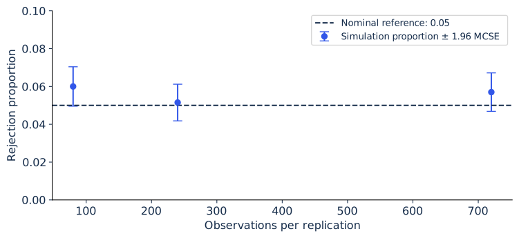
The laboratory generates independent unit-root paths under a specified simple null: zero-drift Gaussian random walks initialized at zero. It fits a DF regression with an intercept, no trend, and no augmented lags. For sample sizes 80, 240, and 720, it repeats the experiment 2,000 times and records the proportion of statistics below $-2.86$.

That threshold is an approximate conventional large-sample 5% reference for the intercept specification. This simulation does not create a calibrated finite-sample critical value for every application. Its purpose is to reveal the sampling variation in a claimed rejection rate and the effect of sample size under this specific data-generating process.

Independent replications require independent draws, and the way a simulation is seeded can remove that independence without any visible error. The laboratory takes every path from one Park–Miller stream with a single documented seed and splits the stream into consecutive blocks of $n$ draws. An earlier version of this laboratory reseeded replication $i$ with $515+i$, and that scheme fails. The generator is multiplicative, so consecutive seeds produce first uniforms that differ by only $48271/(2^{31}-1)$. Over the 200 former replications, the first Box–Muller pair therefore always had a radius between 2.87 and 2.99, while its angle advanced by about 0.53 radians from one seed to the next. Across replications, the first two innovations each had a standard deviation of 2.07 instead of 1. The DF statistic with an intercept does not depend on the first draw of a path, but it does depend on the second, which had about four times its intended variance. Rejection rates computed that way therefore described a walk whose second step had the wrong distribution, drawn in replications that were not independent. Another base seed does not repair the scheme: seeds $2026+i$ over 2,000 replications give a first-draw standard deviation of 1.64. The code now records the standard deviation of the first draw across replications, which should be close to one, and the verification suite fails when it is not.

If $\widehat p$ is a Monte Carlo rejection proportion from $R$ independent replications, its approximate simulation standard error is

$$\operatorname{MCSE}=\sqrt{\frac{\widehat p(1-\widehat p)}R}.$$

With 2,000 replications, a proportion near 0.05 has an MCSE of about 0.005; with 200 replications it would be about 0.015, and differences of a few percentage points would be simulation noise. Increasing observations per replication and increasing replications address different uncertainties. The former changes the statistical experiment; the latter improves how accurately the simulation describes it.

The shared baseline produces rejection rates of 0.060, 0.0515, and 0.057 at $n=80$, 240, and 720, each with an MCSE of about 0.005. The reference script repeats the design with 200,000 replications from NumPy’s generator and obtains 0.054, 0.052, and 0.050, with MCSEs near 0.0005. Each course rate lies within 1.3 of its Monte Carlo standard errors of the corresponding reference rate. The small excess over 0.05 at 80 observations is a genuine finite-sample effect: $-2.86$ is an asymptotic critical value, and the 5% critical value for a sample of that length is slightly more negative. The differences among the course’s three rates are within simulation noise and say nothing about how size varies with sample length.

Dickey–Fuller size at the −2.86 reference: rejection proportions from 2,000 replications per sample size, drawn from one stream, with approximate 95% Monte Carlo error bars.

Why independent random walks can appear related

Suppose $X_t=X_{t-1}+v_t$ and $Y_t=Y_{t-1}+u_t$, with independent innovation sequences. Regressing $Y_t$ on a constant and $X_t$ in levels can generate misleading conventional significance. Each regressor carries a highly persistent random path. Usual stationary-regression laws do not justify the familiar standard-error calculation.

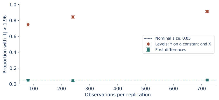
A single realization need not show the problem. The course’s baseline pair has a levels $R^2$ of about 0.0013 and a slope $t$ statistic of about 0.69. We retain that outcome, because the warning concerns the distribution of the procedure across many samples. The laboratory therefore repeats the experiment on 2,000 independent pairs of Gaussian walks for each sample size. The nominal 5% two-sided $t$ test of a zero slope in the levels regression rejects the true null in 74.8%, 84.4%, and 91.3% of replications at $n=80$, 240, and 720, with MCSEs of 1.0, 0.8, and 0.6 percentage points. After differencing, the same test rejects in 4.8%, 4.2%, and 5.0% of replications, close to its nominal size. The reference script’s 200,000 replications give 73.7%, 84.8%, and 91.2% in levels and 5.4%, 5.0%, and 5.0% in differences.

The false-rejection rate rises with the sample. Granger and Newbold (1974) documented the phenomenon by simulation, and Phillips (1986) explained it: in the levels regression the slope estimate converges to a random variable, while the conventional $t$ statistic diverges at rate $\sqrt n$. More data make the misleading inference more confident.

Proportion of 2,000 replications in which the nominal 5% $t$ test rejects a zero slope for independent Gaussian random walks, in levels and in first differences, with approximate 95% Monte Carlo error bars.

Differencing this example gives independent innovations, restoring the intended simple regression setting. But differencing every economic pair indiscriminately can discard a genuine long-run relation. Lecture 11 will construct two $I(1)$ series whose particular linear combination is stationary. Cointegration is the structured exception that must be investigated rather than assumed.

Execute, break, and repair

Run ch06 and inspect df_stat and unit_root_monte_carlo in the full source. Verify that the regression includes an intercept and that the reported statistic uses the lagged-level coefficient. Count the usable observations after differencing. The residual degrees of freedom are the number of usable rows minus the two fitted coefficients.

Deliberately compare the statistic with $-1.96$, the familiar normal threshold. Under this unit-root design, record how often that mistaken rule rejects. Restore the appropriate DF reference and compare. The repair changes the inferential rule; it does not change the fitted coefficient.

Next generate a deterministic trend plus a stable AR disturbance. Compare detrending and differencing using the correct target definition. Detrending estimates deviations from a deterministic path; differencing changes the series into period-to-period changes. Translate forecasts back into the original outcome units before comparing losses.

Finally add a known level break. Report how much the conclusions change when that break is represented explicitly. A unit-root decision should not be used to hide an obvious change in measurement or policy regime.

Worked problem and project audit

A random walk has drift 2, innovation variance 9, and current level 100. Its three-period forecast is 106 and its process-error variance is 27. A stable AR model with innovation variance 9 can also have a three-period variance near 27 when persistence is near one, but its long-horizon variance is finite if $|\phi|<1$. Short-horizon similarity does not establish identical long-run behavior.

For a stationary white-noise series with variance 9, the differenced series has variance 18 and lag-one covariance $-9$. Its lag-one correlation is $-0.5$. Seeing this pattern after differencing is a reason to examine whether the transformation was needed.

During the prototype exchange, audit the partner’s choice of levels, differences, and deterministic terms. Identify what observation would challenge that choice. A defensible audit can conclude that the available sample does not resolve the distinction and recommend robust short-horizon benchmarks. It should not convert an inconclusive test into a confident declaration.

Sources

Dickey and Fuller (1979) derive unit-root estimator distributions. Kwiatkowski, Phillips, Schmidt, and Shin (1992) test the stationarity null. Granger and Newbold (1974) and Phillips (1986) analyze spurious regressions. The practical ARIMA framework is discussed in Forecasting: Principles and Practice.

An economic predictor does not eliminate temporal dependence

Monthly electricity demand depends on weather, calendar patterns, customer counts, and economic activity. An autoregression summarizes persistence without representing those mechanisms explicitly. Dynamic regression adds predictors while retaining a model for unexplained temporal variation:

$$Y_t=x_t'\beta+\eta_t, \qquad \Phi(L)\eta_t=\Theta(L)\varepsilon_t.$$

Here $x_t'\beta$ represents the conditional regression component and $\eta_t$ is a serially correlated disturbance. It is useful to reserve $\varepsilon_t$ for the innovation after that dependence is removed. Treating $\eta_t$ as independent white noise would misstate the uncertainty and waste potential forecasting information.

Different models can place dynamics in different locations. A regression on lagged outcomes and predictors is not generally identical to a static predictor relation with ARMA errors. Their coefficient interpretations and restrictions differ. Write the model in full before translating it to a package formula.

Exogeneity also needs specification. For unbiased or consistent regression estimates, the required relation between predictors and disturbances depends on the model and estimator. A weather variable may be plausibly external to electricity demand, but aggregate economic predictors can react to the same shocks as the outcome. A forecasting association does not establish a causal demand response.

Represent seasonal patterns economically

For monthly observations, deterministic seasonality can be represented by eleven month indicators plus an intercept, or by Fourier terms

$$\sin\!\left(\frac{2\pi kt}{12}\right), \qquad \cos\!\left(\frac{2\pi kt}{12}\right).$$

Low-order Fourier terms produce a smooth repeating annual pattern with fewer parameters. Month indicators allow a more flexible pattern at the cost of more coefficients. At the Nyquist frequency for an even seasonal period, the sine term is identically zero and should be omitted; redundant columns can make the design rank deficient.

Calendar regressors are known in advance. A forecast for next July can use July’s indicator at the origin. Actual next-July temperature is not known. This is an important difference between two variables both associated with seasonality.

A trend in customer count changes the scale of total demand. Modeling sales per customer answers a different question from modeling total sales with customer count as a predictor. If you transform the target, report forecasts and loss in the units the decision requires. A logarithm can improve scale behavior, but $\exp(\mathbb E[\log Y\mid\mathcal I])$ is a conditional median under common lognormal assumptions, not automatically the conditional mean of $Y$.

A nonlinear response to temperature

Heating and cooling mechanisms motivate a piecewise linear response. For a temperature measure $T_t$ and reference $T_0$,

$$H_t=(T_0-T_t)_+,\qquad C_t=(T_t-T_0)_+,$$

with a regression component $\beta_HH_t+\beta_CC_t$. Both slopes can be positive because unusually cold and unusually hot conditions can raise electricity demand through different uses. The threshold is a modeling choice; its interpretation depends on the measured temperature and the energy technology.

The synthetic experiment uses these transformations of a monthly temperature measure. In the observed Texas case, the same transformations are monthly-temperature proxies. They are not sums of daily heating and cooling degree days. A transformation of a monthly mean loses information about the within-month distribution; Lecture 1’s geographic example explains the same noncommutation issue across places.

The research by Chang, Kim, Miller, Park, and Park (2016) models the temperature distribution observed at a higher frequency and a functional demand response. It provides a substantive motivation for treating the distribution of exposure as economically relevant. The introductory piecewise regression here is a simpler teaching model. It does not reproduce that paper’s functional estimator or establish its empirical conclusions. Published article.

Remove an AR(1) error through a transformation

Take the special case

$$Y_t=x_t'\beta+\eta_t,\qquad \eta_t=\rho\eta_{t-1}+\varepsilon_t.$$

Subtract $\rho$ times the lagged regression:

$$Y_t-\rho Y_{t-1} =(x_t-\rho x_{t-1})'\beta+\varepsilon_t.$$

With known $\rho$, appropriate exogeneity, and constant innovation variance, this transformed regression removes the AR(1) disturbance dependence. The intercept column transforms from 1 to $1-\rho$; retaining a column of ones without accounting for this transformation changes the intercept parameterization.

With unknown $\rho$, one feasible approach fits an initial regression, estimates an AR(1) on its residuals, and refits the transformed regression. This is a feasible GLS step. It need not be an exact likelihood estimate, and a single step need not reach the optimum of a joint fitting procedure. Its validity relies on the relevant assumptions and the consistency of the covariance estimate.

The code drops the first observation in the transformation. An alternative treatment can retain it with a stationary initial-state adjustment. Near a unit root, initial-condition handling matters more. Be explicit about which criterion and rows are used before comparing implementations.

Inspect the transformed innovations afterward. If their ACF retains a seasonal pattern, the AR(1) error model has not captured all residual dynamics. If squared innovations cluster, the conditional variance model may need revision. Increasing the mean-model order is not necessarily the correct repair for a variance problem.

Forecast predictors as well as outcomes

The $h$-step forecast combines a regression prediction and an error forecast:

$$\widehat Y_{t+h|t}=\widehat x_{t+h|t}'\widehat\beta +\widehat\eta_{t+h|t}.$$

Known calendar inputs can be inserted directly. Uncertain weather and economic inputs require forecasts, scenarios, or a model that uses only available lags. A prediction conditioned on a stated hot-weather scenario is legitimate; labeling it as an unconditional forecast with realized future weather would misrepresent the information set.

Uncertain predictors contribute to outcome uncertainty. In a simple setting with fixed coefficients and a predictor forecast error $v$, the variance contribution is $\beta'\operatorname{Var}(v)\beta$, plus any relevant covariance with the outcome’s disturbance. Ignoring that term produces overly narrow intervals when weather uncertainty is important.

The code’s hot and cold scenario values compare regression levels at fixed Fourier coordinates. They omit an added forecast of the current residual state and do not assert a future weather probability. Their names explicitly identify them as scenarios. To create a full operational forecast, add the admissible error-state forecast and define the predictor information rule.

Execute, break, and repair

Run ch07. Its declared generating slopes are 0.8 for heating exposure and 1.2 for cooling exposure, and its error persistence is 0.6. The shared realization estimates error persistence near 0.62. Feasible GLS produces slopes near 0.781 and 1.242. These results recover the broad response in this controlled setting while retaining finite-sample deviations.

Examine the source’s design matrix. Verify that the Fourier inputs are known calendar functions, that the intercept is transformed along with every other column, and that the same rows enter both sides of the transformed regression. Compare the innovation ACF before and after the repair. A small remaining lag-one value is encouraging for this simulation but is not proof of independence.

Break the procedure by adding actual future temperature to a historical forecast without a scenario label. Apply the origin’s availability rule and identify the inadmissible input. Repair it by using a declared seasonal temperature expectation, a separately evaluated weather forecast, or lagged predictors. Retain the resulting loss comparison even if performance worsens: an honest operational forecast can be less accurate than an impossible retrospective one.

Worked problem and audit connection

Let $Y_t=10+2X_t+\eta_t$ and $\rho=0.5$. If $(Y_t,Y_{t-1})=(20,16)$ and $(X_t,X_{t-1})=(4,3)$, transformed outcome is 12 and transformed predictor is 2.5. The transformed intercept is $10(1-0.5)=5$, so the regression component is $5+2(2.5)=10$. The transformed innovation is 2. Keeping an untransformed intercept of 10 would produce the wrong decomposition.

Suppose the current fitted error is 3, its persistence is 0.5, and next month’s regression component under a stated weather scenario is 100. The one-step scenario forecast is $100+0.5(3)=101.5$. At two steps, the residual-state contribution is $0.5^2(3)=0.75$. The scenario’s weather path must still be supplied separately.

For Project 2, distinguish a misspecified error process from a predictor-timing violation. Each calls for a different repair. A reviewer should identify the exact affected forecast origins, explain why the issue matters, and replicate the consequence using a controlled change.

Further reading

Forecasting: Principles and Practice on dynamic regression and forecasting with future regressors supply practical context. The temperature-distribution motivation comes from Chang and colleagues (2016).

Write the state and observation mechanisms separately

A scalar state-space model is

$$S_t=\phi S_{t-1}+\eta_t,\qquad Y_t=S_t+\nu_t,$$

where state innovations have variance $q$ and observation disturbances have variance $r$. In the elementary Gaussian version, both disturbance sequences are independent over time and independent of each other. The model separates an evolving economic quantity from a noisy observation of it.

The core exercise treats $\phi,q,r$ as given. Estimating all three adds identification, optimization, and initial-state questions. Those are useful extensions, but a working filter should first be understood with a transparent specified model. A smooth output alone cannot tell us whether its variance parameters are economically defensible.

If the state and observation share the same unit, $q$ and $r$ have squared units. A model with observation loading $\lambda$ would require consistent scaling: $Y_t=\lambda S_t+\nu_t$. The loading establishes how state units translate into indicator units. Without a normalization, latent scales can be arbitrary.

Predict the state before observing the new record

Let $m_{t-1}$ be the filtered mean of $S_{t-1}$ and $P_{t-1}$ its filtered variance, conditional on observations through $t-1$. The transition equation gives the prior prediction

$$a_t=\phi m_{t-1},\qquad V_t=\phi^2P_{t-1}+q.$$

The observation prediction is also $a_t$ because the loading is one and observation noise has mean zero. Its prediction-error variance is $V_t+r$. Define the observation innovation $v_t=Y_t-a_t$. This is an error in predicting the observed indicator; it is different from the unobserved state innovation $\eta_t$.

The new observation contains information about the state because $\operatorname{Cov}(S_t,Y_t\mid\mathcal I_{t-1})=V_t$. Under Gaussian conditioning, the state update is

$$K_t=\frac{V_t}{V_t+r},\qquad m_t=a_t+K_tv_t,\qquad P_t=(1-K_t)V_t.$$

The Kalman gain $K_t$ is dimensionless and lies between zero and one when $V_t\ge0$ and $r>0$. A noisy indicator gets a small weight; a precise indicator gets a large weight. The posterior mean is a weighted combination of the prior state estimate and the new observation.

The variance update follows from the same conditional-Gaussian formula: $P_t=V_t-V_t^2/(V_t+r)=V_tr/(V_t+r)$. It cannot exceed the prior variance. This is an analytic check that an implementation should preserve up to floating-point tolerance.

Check limiting cases

As $r\to\infty$, $K_t\to0$, and the observation contributes almost nothing. As $r\to0$ with positive prior variance, $K_t\to1$, the filtered state approaches the observed value, and posterior variance approaches zero. If $q$ increases, the prior becomes less precise and the new observation generally receives more weight.

If $\phi=0$, the prior state does not depend on the previous filtered state. If $q=0$, the state evolves deterministically from its initial uncertainty; repeated observations can progressively reduce uncertainty about that initial condition. Degenerate combinations require careful implementation to avoid division by zero or an unjustified stationary initialization.

For $|\phi|<1$, a stationary prior variance is $q/(1-\phi^2)$. The supplied code initializes the previous state mean at zero and variance at this stationary value, then applies the transition before the first observation. That convention implies the same stationary prior variance at the first observation. A diffuse prior or an economically informed initial state is a different specification.

Handle a missing observation by skipping its update

If $Y_t$ is missing, the state still evolves. Calculate $a_t$ and $V_t$, then set $m_t=a_t$ and $P_t=V_t$. There is no measurement update because no observation has arrived. Imputing $Y_t=0$ would instead treat zero as a real observation and could pull the state sharply toward it.

A run of missing observations increases uncertainty toward the transition model’s unconditional variance when the stable model applies. In an application, missingness may itself be informative. A measurement system that fails preferentially during extreme events violates the simple missing-at-random interpretation. The filter recursion can handle a missing input computationally while the underlying statistical assumptions remain questionable.

The data clock still applies. If the observation describes period $t$ but arrives later, update the model when it becomes available, using a properly specified delayed-observation system if necessary. Merely labeling it $t$ does not authorize an earlier update. The scalar exercise assumes observations arrive in their sequence at the stated dates.

Retrospective smoothing uses the future

After observing the entire sequence through $T$, a smoother estimates $S_t$ conditional on $\mathcal I_T$. Write its mean as $m_{t|T}$ and its variance as $P_{t|T}$; in this notation the filtered quantities $m_t$ and $P_t$ are $m_{t|t}$ and $P_{t|t}$. The scalar Rauch–Tung–Striebel recursion starts from $m_{T|T}=m_T$ and $P_{T|T}=P_T$ and moves backward:

$$J_t=\frac{P_t\phi}{V_{t+1}}, \qquad m_{t|T}=m_t+J_t(m_{t+1|T}-a_{t+1}),$$ $$P_{t|T}=P_t+J_t^2(P_{t+1|T}-V_{t+1}).$$

The backward correction uses what later observations reveal about earlier states. Under the specified Gaussian model, conditioning on more observations weakly reduces state uncertainty. The code checks that each smoothed variance $P_{t|T}$ is nonnegative and no larger than the corresponding filtered variance $P_t$. In the source, ms and Ps hold $m_{t|T}$ and $P_{t|T}$.

A smoother can improve historical state estimation while being unavailable for a real-time decision at that historical date. This is the model-based counterpart to Lecture 5’s centered average. Use filtered states to evaluate an earlier decision; use smoothed states to describe a retrospective reconstruction with its later information set stated.

The innovation likelihood and its limits

With specified Gaussian parameters, observation innovations give a log-likelihood contribution

$$\ell_t=-\frac12\left[\log(2\pi)+\log(V_t+r)+\frac{v_t^2}{V_t+r}\right].$$

Summing over observed dates supplies a likelihood objective for parameter estimation. Missing dates contribute no observation density while still changing the state prediction. Optimizing this objective requires admissible variance parameters, an initial-state convention, and checks for local solutions.

The standardized innovations $v_t/\sqrt{V_t+r}$ should have the assumed mean, variance, and dependence under a correctly specified model. Persistent correlation suggests missing state dynamics; unusual tails suggest a distributional mismatch; a variance shift can reflect a changing instrument or a changing state process. Estimating parameters does not eliminate the need to inspect these implications.

Known synthetic state, filter, and retrospective smoother. The shaded band uses the specified Gaussian filter variance; one observation is deliberately missing.

Execute and replicate independently

Run ch08. The generator uses $\phi=0.8$, $q=0.25$, and $r=1$, then deliberately removes one observation. The shared realization gives filter RMSE around 0.562 and smoother RMSE around 0.496 against the known simulated state. This comparison is possible because the simulation reveals its state; observed economic data generally do not.

The missing date’s filtered variance exceeds the preceding posterior variance. That result follows from skipping the update in this setting; the exact magnitude depends on parameters and prior uncertainty. Inspect the missing-value branch in every implementation and confirm it does not insert a zero observation.

Apply the future-mutation test by adding 10 to observations after index 180. The filter at 180 remains unchanged. The smoother at 180 changes materially because its later information changes. Freeze the parameter values during this comparison; otherwise a full-sample parameter refit can also change earlier filtered estimates.

Independently reproduce the first three updates by hand or in a short script before reading the implementation’s output. On the course’s audit day, protect time for this replication. A student who only reproduces the final graph has not demonstrated that the prediction and update steps are understood.

Worked update and project repair

Suppose the prior state mean is 10 and variance is 4, observation variance is 1, and the new indicator is 13. The gain is $4/(4+1)=0.8$, the posterior mean is $10+0.8(3)=12.4$, and posterior variance is $(1-0.8)4=0.8$. The observation moves the state toward 13 but does not eliminate uncertainty.

If observation variance instead equals 16, the gain is $4/20=0.2$, posterior mean is 10.6, and posterior variance is 3.2. The noisier observation contributes less information. If the observation is missing, the prior mean 10 and variance 4 remain the current estimate after the prediction step.

For Project 2, a measurement repair should state whether it changes the indicator, the state transition, the observation variance, or the admitted information. Do not replace a centered feature with a smoother and claim to have removed future dependence. An admissible repair must preserve the appropriate decision clock.

Sources

Kalman (1960) is the foundational filtering paper. Rauch, Tung, and Striebel (1965) derive the fixed-interval smoother. QuantEcon’s linear state-space lecture supplies a broader treatment.