Predictable risk with an unpredictable return

The conditional mean and conditional variance can behave differently

Let a return be $R_t=\mu_t+u_t$, with $\mathbb E[u_t\mid\mathcal I_{t-1}]=0$. Zero predictable mean does not imply constant risk. Write

$$u_t=\sqrt{h_t}z_t,\qquad \mathbb E[z_t\mid\mathcal I_{t-1}]=0,\qquad \mathbb E[z_t^2\mid\mathcal I_{t-1}]=1.$$

Then $h_t=\operatorname{Var}(u_t\mid\mathcal I_{t-1})$. It is known at the forecast origin under the specified variance recursion, while the next standardized shock is not. A sequence can have little autocorrelation in returns and appreciable dependence in squared returns.

Financial returns provide a familiar application, but the distinction also matters for economic quantities whose uncertainty changes across seasons, regimes, or measurement systems. A larger mean model does not automatically explain conditional variance dynamics.

Before estimating volatility, define the return. A decimal return of 0.01 is a one-percent return; a percentage-point return of 1 represents the same change on a different numerical scale. Log returns and simple returns are also different transformations. State the definition and use it consistently in means, variances, and risk thresholds.

ARCH and GARCH recursions

An ARCH(1) variance is $h_t=\omega+\alpha u_{t-1}^2$. A GARCH(1,1) adds lagged variance:

$$h_t=\omega+\alpha u_{t-1}^2+\beta h_{t-1}.$$

Sufficient elementary restrictions for positive conditional variance are $\omega>0$, $\alpha\ge0$, and $\beta\ge0$. For a finite unconditional second moment in the standard model, impose $\alpha+\beta<1$. Strict stationarity can have a different condition involving an expected log; the finite-variance restriction used here is stronger than some stationarity conditions and should be named accurately.

The units agree: $h$, $u^2$, and $\omega$ have squared return units; $\alpha$ and $\beta$ are dimensionless. The lagged squared error updates risk after a large realized surprise, while the lagged variance carries previously assessed risk forward.

Taking expectations under a finite stationary second moment gives

$$\overline h=\omega+(\alpha+\beta)\overline h, \qquad \overline h=\frac{\omega}{1-\alpha-\beta}.$$

As $\alpha+\beta$ approaches one with fixed $\omega$, unconditional variance increases. At the boundary, that finite-variance formula no longer applies. A routine that reports a negative unconditional variance for an inadmissible parameter set has failed a basic domain check.

Forecast conditional variance

At date $t$, after observing $u_t$, the one-step variance forecast is

$$h_{t+1|t}=\omega+\alpha u_t^2+\beta h_t.$$

For later horizons, use $\mathbb E[u_{t+j}^2\mid\mathcal I_t]=h_{t+j|t}$ under the model. This yields

$$h_{t+k|t}=\overline h+(\alpha+\beta)^{k-1}(h_{t+1|t}-\overline h),\qquad k\ge1.$$

Variance reverts toward its long-run level at persistence $\alpha+\beta$. At $k=1$, the exponent is zero and the expression returns the known one-step forecast. If $\alpha=\beta=0$, risk is constant at $\omega$.

Variance of a multi-period cumulative return is the sum of the conditional variance forecasts when the mean-adjusted returns form the required martingale-difference sequence and cross-covariances vanish. The square-root-of-time rule requires constant per-period variance and the appropriate independence or orthogonality assumptions. Applying it mechanically during changing volatility can misstate multi-period risk.

Estimate a declared objective

Under conditional Gaussianity, the negative log-likelihood apart from constants is

$$Q(\theta)=\frac12\sum_t\left[\log h_t(\theta)+\frac{u_t^2}{h_t(\theta)}\right].$$

The supplied code minimizes the average expression without the factor one-half over a declared admissible grid. Multiplying an objective by a positive constant does not change its minimizer. The grid estimator is coarse and transparent; it is not a substitute for a carefully checked continuous optimizer when precise estimation is required.

Under suitable conditions, Gaussian quasi-likelihood can estimate variance parameters without exactly Gaussian innovations. Standard errors then require the appropriate robust treatment. The core grid example supplies no maximum-likelihood standard errors and makes no inferential claim based on a Hessian it has not computed.

The variance recursion is initialized at its candidate unconditional variance. Alternative backcasts or initial values can change short-sample objectives. Retain the initial rule, estimation dates, mean-model treatment, convergence diagnostics, and parameter restrictions when comparing package outputs.

A risk quantile needs a distribution

If $z_{t+1}$ is standard normal and the conditional mean is $\mu_{t+1}$, the conditional return quantile is

$$q_p=\mu_{t+1}+\sqrt{h_{t+1|t}}\,\Phi^{-1}(p).$$

For $p=0.05$, the standard-normal multiplier is approximately $-1.645$. A variance forecast alone does not establish that tail quantile. Heavy-tailed or asymmetric standardized shocks require a different distributional model or a justified empirical quantile procedure.

Value at Risk needs a sign and loss convention. A negative return quantile can correspond to a positive loss threshold. Define whether the reported object is a return, a dollar loss, or a portfolio loss; identify the horizon and confidence level. Expected shortfall is a different tail summary and cannot be inferred by merely renaming the same quantile.

Evaluate risk forecasts using actual subsequent outcomes. Count and date threshold exceedances; inspect clustering as well as their overall frequency. A model can have the desired average exception rate while failing during the periods when risk decisions matter most. Repeatedly changing a threshold after inspecting its exceptions invalidates a clean later-target comparison.

Scaling is an exact audit

If returns are rescaled as $u_t^*=a u_t$, an equivalent variance model has

$$h_t^*=a^2h_t,\qquad \omega^*=a^2\omega,\qquad \alpha^*=\alpha,\quad\beta^*=\beta.$$

Moving from percentage-point returns to decimal returns sets $a=0.01$, so variance and $\omega$ divide by 10,000. Standard deviations and quantiles divide by 100. A failure of these transformations reveals a units error independent of whether the model fits well.

The code tests this identity directly using the same residuals and parameters. It also deliberately presents an inadmissible parameter set with $\alpha+\beta>1$ and checks that the finite-variance routine rejects it. These tests establish computational invariants. They do not establish that the fitted variance model describes real financial markets.

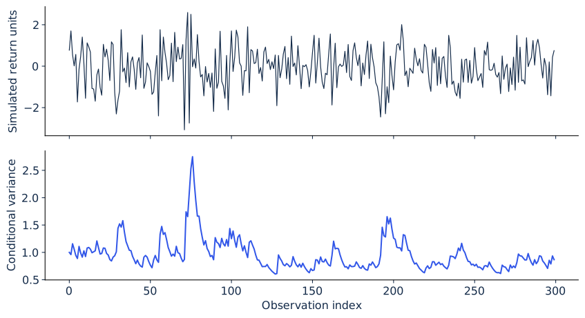
Simulated returns and their generating conditional variance. Return surprises can be unpredictable while risk varies.

Execute, break, and repair

Run ch12. The synthetic process has $\omega=0.1$, $\alpha=0.1$, and $\beta=0.8$, giving unconditional variance one. The declared coarse grid selects $(0.2,0.1,0.7)$ on this realization. Including the true parameters in a finite-sample grid does not guarantee that they will minimize the realized objective.

The squared-return lag-one correlation is around 0.151, while the squared standardized-residual correlation is around 0.012. This is consistent with the fitted variance recursion removing much of the visible clustering in the chosen realization. Inspect additional lags and tail behavior before treating that diagnostic as a complete verdict.

Break the risk calculation by using $h_t$ in place of $h_{t+1|t}$ after the latest residual has arrived. The mistake ignores the newest variance update. Repair it with the one-step recursion and compare the threshold. Then divide returns by 100 without rescaling $\omega$; identify the resulting units inconsistency and correct it.

Worked risk forecast and audit repair

Let $\omega=0.2$, $\alpha=0.1$, $\beta=0.8$, current variance $h_t=2$, and current residual $u_t=3$ in percentage points. Next variance is $0.2+0.1(9)+0.8(2)=2.7$, and next standard deviation is $\sqrt{2.7}\approx1.643$ percentage points. Under a zero-mean normal specification, the 5% return quantile is approximately $-2.703$ percentage points.

Long-run variance is $0.2/(1-0.9)=2$. The two-step variance forecast is $2+0.9(2.7-2)=2.63$. The model expects risk to decline gradually from the elevated current forecast. With decimal-return units, next variance is 0.00027 and the quantile is approximately $-0.02703$.

Project 2’s repair can address a variance error without changing the entire mean model. Show which risk decision changes and which assumptions remain unresolved. Project 3 should evaluate the repaired procedure on later outcomes, preserving the loss and threshold rules chosen before the continuation data are examined.

Sources

Bollerslev (1986) introduces GARCH. The arch package’s official volatility-model documentation describes mean, variance, and distribution components.