7 Results
7.1 The headline FE decomposition
Estimated by scripts/run_regressions.py; results are in data/processed/regressions/main_table.{csv,md}. Outcome variable is project-level leverage, winsorized at [1, 20]. Standard errors in parentheses; M0–M3 use HC1, M4–M5 cluster at the CDE level.
| M0 | M1 | M2 | M3 | M4 | M4-Q | M5 | |
|---|---|---|---|---|---|---|---|
| rural (\hat\beta) | −0.262*** | −0.249*** | −0.186*** | −0.172** | −0.047 | −0.001 | 0.091 |
| (SE) | (0.060) | (0.061) | (0.061) | (0.067) | (0.101) | (0.008) | (0.621) |
| year FE | — | ✓ | ✓ | ✓ | ✓ | ✓ | ✓ |
| QALICB-type FE | — | — | ✓ | ✓ | ✓ | ✓ | ✓ |
| state FE | — | — | — | ✓ | — | — | — |
| CDE FE | — | — | — | — | ✓ | ✓ | ✓ |
| R^2 | 0.002 | 0.015 | 0.022 | 0.039 | 0.131 | — | 0.132 |
| N | 8,024 | 8,024 | 8,024 | 8,024 | 8,024 | 8,024 | 8,024 |
Stars: *** p<0.01, ** p<0.05, * p<0.10.
7.2 Reading the layered specs
M0 → M1 (+ year FE). The coefficient barely moves: −0.262 → −0.249. The 2001–2022 macro credit cycle is not what drives the rural gap.
M1 → M2 (+ QALICB-type FE). Substantial shrinkage: −0.249 → −0.186. The “rural projects are more NRE-skewed” composition story explains roughly 25% of the M1 gap. Composition matters but is not dominant.
M2 → M3 (+ state FE). Small additional shrinkage: −0.186 → −0.172. State capital-market depth explains a modest additional fraction.
M3 → M4 (+ CDE FE). The dominant decomposition step: −0.172 → −0.047, and the coefficient is no longer statistically distinguishable from zero (p = 0.64). This is the headline result. The reduction from M3 to M4 — from −0.172 to −0.047 — is the between-CDE selection component. It accounts for roughly 73% of the M3 gap and roughly 80% of the M0 gap.
The median spec (M4-Q) confirms. The median within-CDE rural effect is −0.001× — essentially zero. At the median, when the same CDE does both metro and non-metro deals in the same year and the same project type, there is no rural leverage penalty.
7.3 Interpretation in plain English
The aggregate rural leverage gap of 0.26× (mean) or 0.12× (median) is real. But when we compare like to like — same CDE, same year, same project type — the gap essentially disappears. The same intermediary, deploying the same federal credit, produces the same leverage whether it deploys in a rural or urban tract.
Therefore the aggregate gap is almost entirely between-CDE selection: rural-specialist CDEs are systematically less effective at private- capital mobilization than urban-specialist CDEs, not because rural markets are deficient, but because the institutions allocated to rural tracts have different organizational capabilities. The federal program isn’t catalyzing less private capital rurally because the rural market is broken; it’s catalyzing less private capital rurally because the CDEs deploying there happen to be less skilled at leverage.
This is a far sharper, more policy-actionable, and more publishable finding than “rural deals leverage less.”
7.4 Rural × QALICB-type interaction
The M5 specification interacts the rural indicator with QALICB-type dummies (CDE-to-CDE is the omitted category). Coefficient estimates:
| term | \hat\beta | (SE) | p |
|---|---|---|---|
rural |
0.091 | (0.621) | 0.883 |
rural × NRE |
−0.085 | (0.647) | 0.895 |
rural × RE |
−0.397 | (0.648) | 0.540 |
rural × SPE |
−0.046 | (0.642) | 0.943 |
The interaction terms are imprecisely estimated because within-CDE-by- type cells become small once both CDE FE and the interaction are included. The point estimates suggest the within-CDE rural penalty is largest in real estate (consistent with the descriptive Chapter 3 figure), but the standard errors do not allow strong inference about type-specific heterogeneity in the within-CDE channel.
7.5 The bunching diagnostic
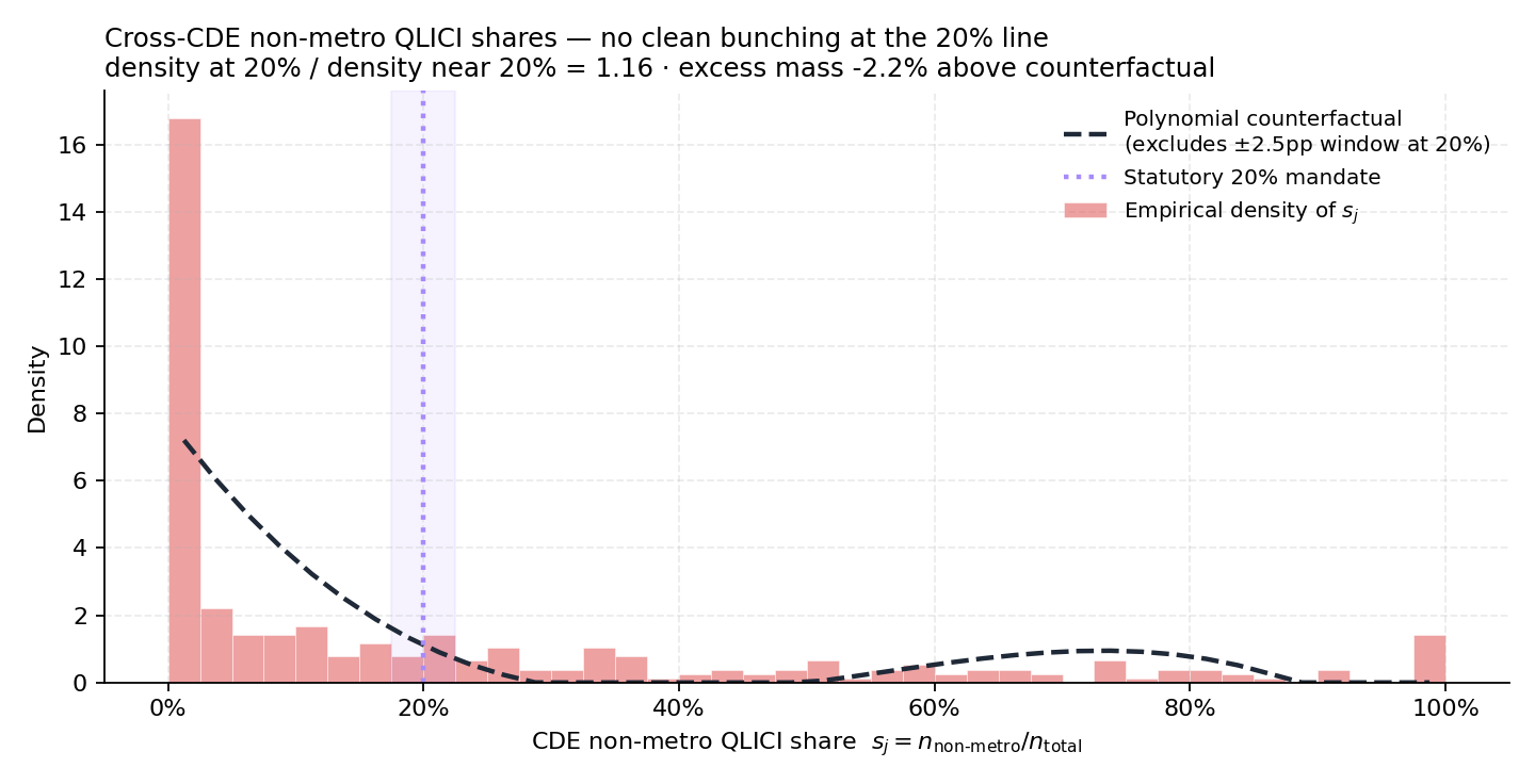
Of 310 CDEs with at least five QLICI transactions, the cross-CDE distribution of cumulative non-metro shares does not show evidence of bunching at the 20% mandate. The empirical mass in the [17.5%, 22.5%] window is 0.0274; the counterfactual mass under a degree-3 polynomial fit (excluding the window) is 0.0280; the excess mass is essentially zero (slightly negative).
The visual shows why: the cross-CDE distribution is bimodal, with a heavy mode at 0% (urban-specialist CDEs) and a smaller mode at 30–50% (rural-specialist CDEs). The 20% line falls in the low-density valley between the modes, not on a peak.
7.5.1 Two interpretations
The mandate likely binds at the allocation-award stage, not at the cumulative-deployment stage. CDFI requires CDEs to commit to ≥20% non-metro deployment in their competitive applications, but the deployment unfolds over several years. We see only the realized deployments, not the awarded commitments. CDEs may bunch at 20% in their applications but realize a different share over the deployment window.
The CDE distribution has sorted bimodally — into urban-specialist and rural-specialist groups, with relatively few “balanced” intermediaries. The 20% line is not naturally attractive because few CDEs operate in a regime where 20% would be the binding constraint.
Both interpretations are consistent with the data. The first is more about regulatory mechanics; the second is more about industry structure. The substantive finding is itself novel — the literature has assumed the 20% mandate binds; we provide the first empirical evidence that, at the realized-deployment level, it does not show up as a bunching signature.
7.6 Robustness (in progress)
The companion robustness battery being completed for the working-paper draft includes:
- M0–M4 on the unwinsorized
leverage_ratio - M0–M4 restricted to projects with leverage ≤ 5×
- M0–M4 sub-period split (pre-2010 vs. post-2010)
- M0–M4 restricted to the top-50 CDEs (where CDE FE is most precisely estimated)
- Two-way clustering on (CDE, tract)
- USDA RUCA-based continuous rurality (in place of binary metro flag)
Results will be reported in §5.3 of the formal paper draft and reflected in the data tables here as the analyses complete.