The New Markets Tax Credit is the US federal program whose mechanics most closely
match the "blended finance" story you want to tell. The federal government offers
investors a 39% tax credit (claimed over 7 years) in exchange for
putting their equity into a certified Community Development Entity (CDE).
The CDE is a regulated intermediary — usually a bank subsidiary or a nonprofit
community-development financial institution — that re-deploys the money as loans
or equity into qualifying businesses and projects located in low-income census
tracts. Those projects are called QALICBs.
What we observe is the CDE → QALICB flow (the QLICI): who got how much,
where, in which year, and what the total project cost was. The investor-side flow
(QEI, and the tax credit they claim) is upstream and off the public data release.
The rural mandate
The NMTC statute requires CDEs to direct at least 20% of their QLICIs to
non-metropolitan census tracts. That creates a testable prediction: CDEs will
bunch against the 20% line unless they have a strong pull to go further.
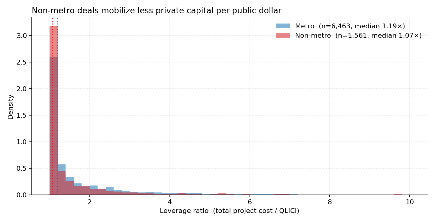
Leverage, as we measure it here
The leverage ratio of a project is total project cost / QLICI. If a $5M
project received a $1M QLICI, it leveraged the federal dollar 5×, meaning $4 of
non-federal capital showed up per $1 of credit. That's the mobilization number.
Why this question is identifiable
Two sharp discontinuities the law gives us for free:
(1) tracts qualify only if poverty ≥ 20% or median family income ≤ 80% of
area median — an RDD cutoff; (2) the 20% rural mandate — a bunching test.
See DATA_DICTIONARY.md for every
column and PROVENANCE.md for SHA-256
hashes, license terms, and a step-by-step recreate-from-scratch recipe.
Every NMTC project, on an Earth map
Each dot is one project, placed at its 2020-census-tract centroid.
Metro · Non-metro.
Dot size ∝ √(QLICI $).
Hover for detail. Scroll-zoom to explore.
— projects · —
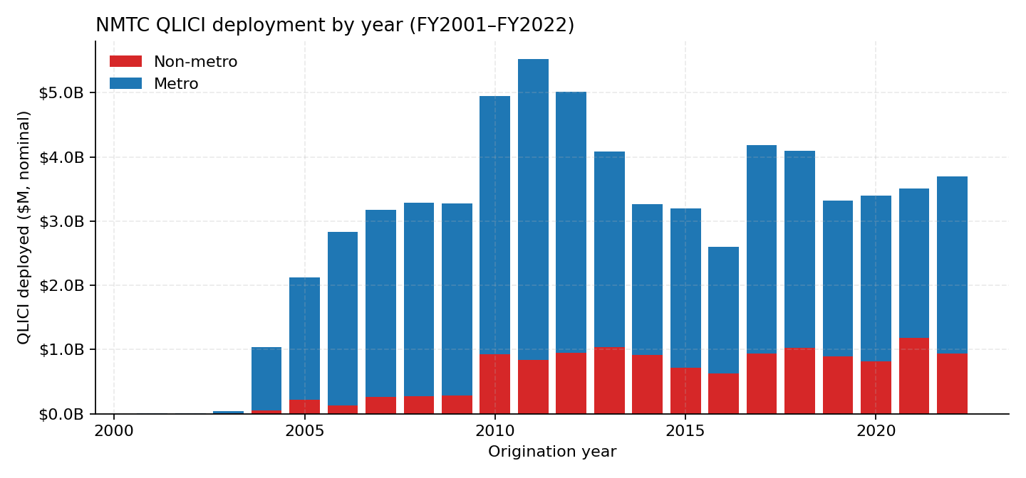
Deployment through time
The program ramped from almost nothing in FY2001 to ~$5 B/yr through the 2010s,
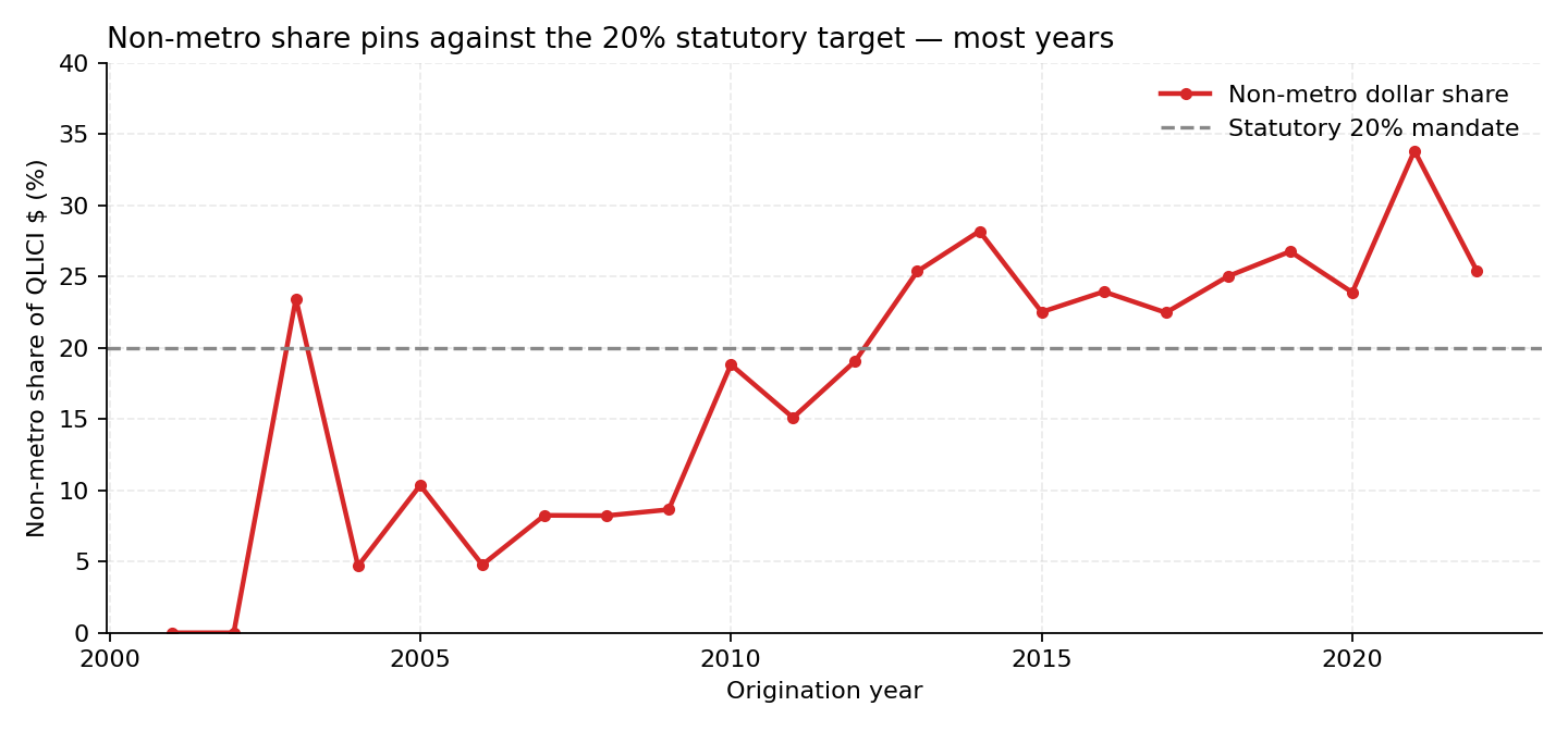
then settled into a $3–4 B/yr steady state. The stacked bar shows metro vs. non-metro
dollar share; the panel below it pulls the non-metro share out as a line, against
the 20% statutory mandate.
Fig 1 · Annual QLICI deployment, metro vs non-metro stacked.Fig 2 · Non-metro dollar share pins the 20% line in most pre-2013 years,
hovers slightly above it thereafter. Classic mandate-binding behavior.
The leverage gap
This is the empirical headline of the first-look brief. Non-metro projects sit
heavier on the 1.0× floor (nearly 100% NMTC-financed, zero private capital
mobilized) while metro projects show a fatter right shoulder (more private debt
and equity stacked on top).
Fig 3 · Leverage-ratio density, metro vs non-metro.
Median metro 1.19× vs. non-metro 1.07×. The gap is small at the median but
the shape tells the story: rural deals rarely stack private capital on top.
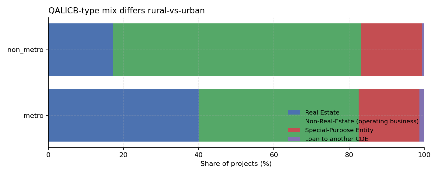
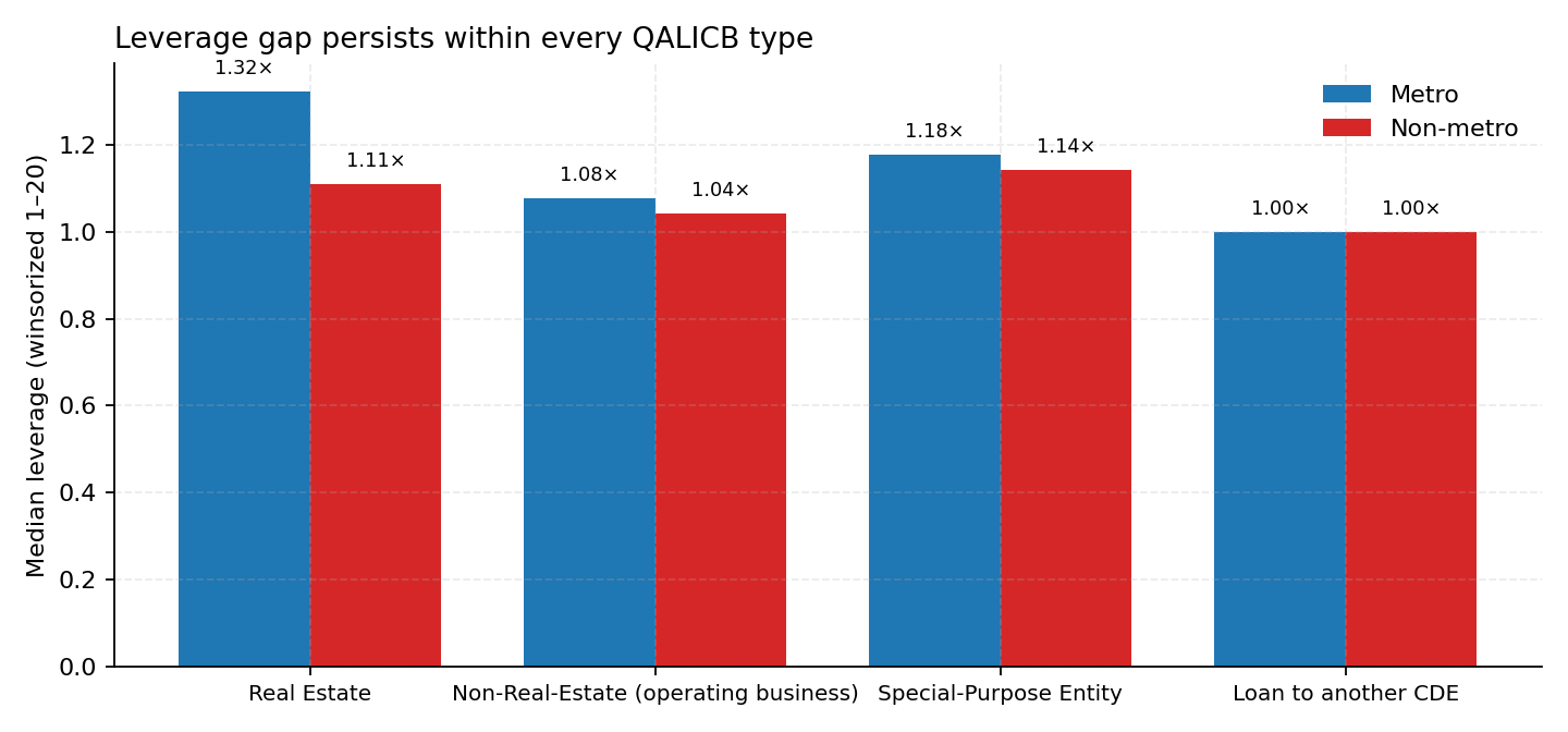
Fig 4 · Metro skews Real-Estate (~40%); non-metro skews operating-business NRE (~65%).
So the leverage gap could be a composition story — except…Fig 5 · …the gap persists within every QALICB type.
It's not composition. It's something about deploying the credit rurally.
CDE-level heterogeneity — the mechanism candidate
Same credit, same 39% federal subsidy, same statute. But the top-20 CDEs — which
together account for more than half of all NMTC dollars — deploy wildly differently
along the rural margin. This is where the paper probably lives.
CDE
QLICI $M
tx
non-metro share
deployment
Sorted by non-metro share (descending). The top row — Rural Development Partners LLC
at ~80% non-metro — and the bottom few (ESIC, Consortium America, Capital Impact) at
<5% are the same federal instrument deployed to different worlds. A within-CDE
fixed-effects specification absorbs that selection.
What the econometrics look like
Four specifications, all identifiable from the public release plus a routine
Census-tract merge.
and the brief reports $\hat\beta \approx -0.26$ (mean) or $-0.12$ (median,
via a quantile regression). But that's contaminated by which CDE
deploys where and what type of project. The fixed-effects version:
with $\gamma_{c(i)}$ a CDE fixed effect, $\delta_{t(i)}$ origination-year,
and $\eta_{q(i)}$ a QALICB-type fixed effect. The quantity of interest is
whether $\hat\beta$ survives the CDE fixed effect — i.e. does the same
CDE mobilize less private capital in non-metro than in metro?
3 · The LIC-eligibility regression discontinuity
A census tract is NMTC-eligible if either condition holds:
where $Y_\ell$ is, say, tract-level NMTC dollars per capita or mean leverage.
$\hat\tau_{R=\text{metro}}$ vs. $\hat\tau_{R=\text{non-metro}}$ is exactly the
"does the policy bite differently in rural markets" question.
4 · The 20% mandate — a bunching test
Let $s_j$ be CDE $j$'s realized non-metro share of QLICIs. The statute requires
$s_j \ge 0.20$. Under no-mandate counterfactual, $s_j$ would be smooth around
$0.20$. Under a binding mandate, we expect a visible mass at $s_j = 0.20$.
Formally, compare the empirical density $\hat f(s)$ to a polynomial fit that
excludes a window around the cutoff:
$B > 0$ is the "excess mass" due to the mandate — standard Chetty et al. (2011) /
Kleven (2016) machinery. CDEs that exceed the mandate voluntarily reveal
willingness-to-deploy rurally; CDEs that pin the mandate are constrained.
The marginal rural project identifies off the constrained CDEs.
5 · Putting it together
The empirical paper is short: (2) establishes that the rural gap isn't a
composition artefact (CDE FE absorbs identity, QALICB FE absorbs type);
(3) shows that the RDD treatment effect differs between metro and
non-metro (the interaction we care about); (4) validates the identifying
assumption by showing CDEs bunch exactly where the law says they would.
Where to go next — three moves
Census-tract merge (this week). Join tract FIPS to 2016–2020 ACS
poverty + MFI + population + USDA RUCA codes. That gives us the RDD running
variable ($P_\ell - 0.20$) and a continuous rurality gradient (RUCA 1–10)
instead of the binary metro flag.
CDE-type classification (this week). Hand-classify the top 50
CDEs by institutional form — bank subsidiary / nonprofit CDFI / for-profit
specialized / government. Turns "CDE variation" from a name into a
structural variable we can interact with rural.
First-look figure (next week). Binned scatter of project-level
leverage vs. tract poverty rate, metro and non-metro overlaid. If the
discontinuity is visible at the 20% poverty threshold for both subgroups
but the rural slope is flatter, the paper is real.